Modern AI Accelerators: GPU / TPU Systems Course / Core track / Topic 3 / The Evolution of Attention 🌐 中文

The Evolution of Attention

In 2020, GPT-3 could hold 2048 tokens. Today's models hold 1M.
The last six years of attention are the story of how that 512× was bought.

One complete story, in chronological order: how a chain got cut, what the cut left unpaid, how four groups paid it four ways, and why it all ended back at the fixed-size notepad. Many figures, few words, plain language.

Prereqs Topic 1 · Topic 2 Read front to back Derivations and measurements not covered

Course author Chris Yang·Google Cloud AI Infra architect

This lecture has instructor notes.

They cover how to teach it: each segment's goal, where to pause, common misconceptions, likely questions. The content itself is this page.

Two uses. Presenting: teach from them; lines, figure cues and timing are written out. Self-study: give the notes to an AI and get a TA who knows the lecture and how to teach it; let it walk you through.

Section 0

The eight years at a glance
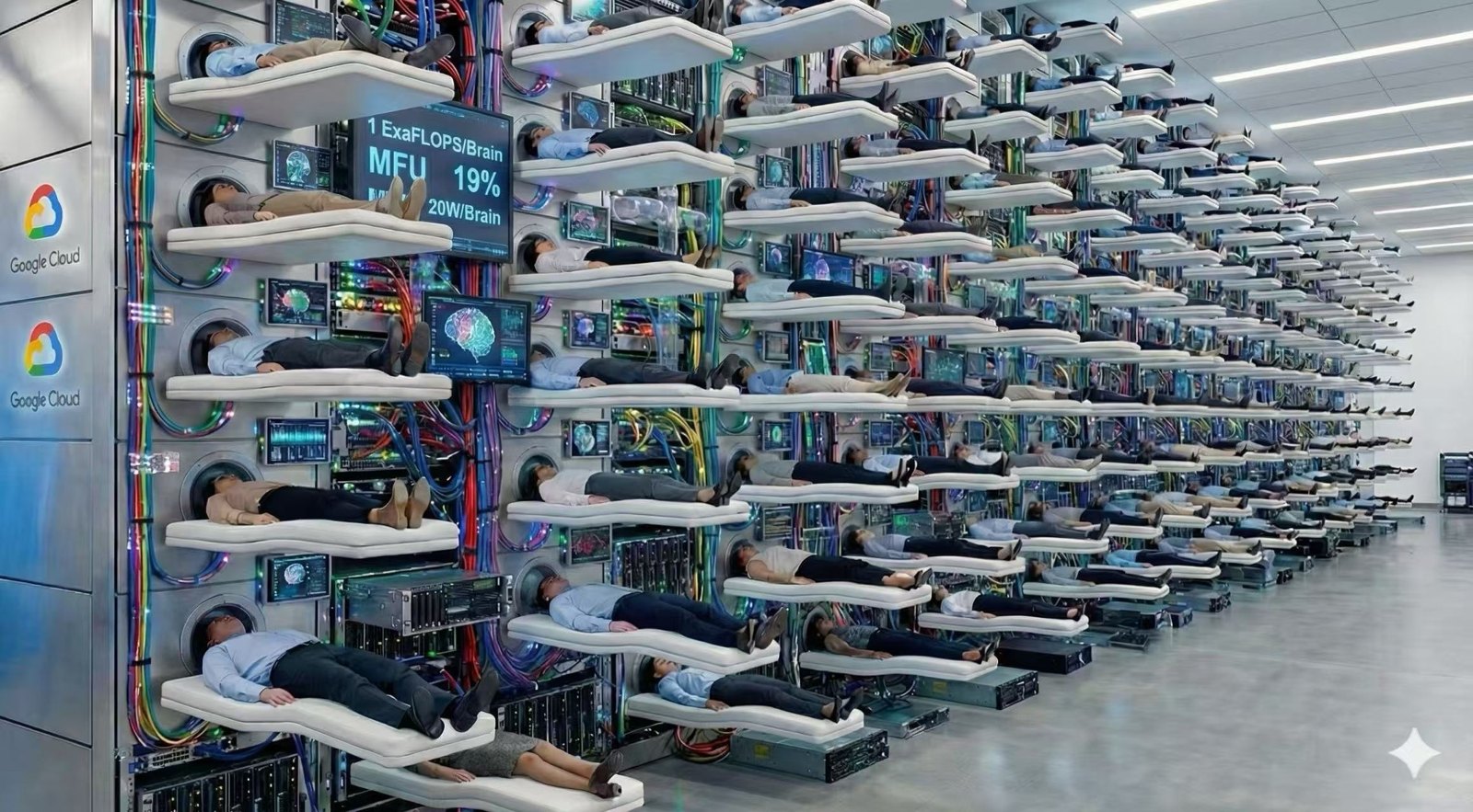
A data-center rack filled with people lying in the slots; the screen reads 1 ExaFLOPS/Brain, MFU 19%, 20W/Brain
⭐⭐ This lecture's two threads: how models remember and how people remember. Every memory-saving trick leans the same way.
⛔ Of its three numbers, only one holds up. Check them all first: this course's rule.

⛔⛔ Minute one: audit these numbers.

  • 20 W/brain: holds up. Physiologically grounded: the brain is ~2% of body weight yet burns 20% of its metabolism. 10-odd to 20 W is citable.
  • 1 ExaFLOPS/brain: not usable as a number. Public estimates of the brain's “equivalent compute” span 10¹² to 10²⁸, sixteen orders of magnitude. 1 ExaFLOPS is one point, not a consensus.
  • MFU 19%: a joke. MFU's denominator is the chip's rated peak, and a brain has no spec sheet, so it isn't even defined.

⭐⭐ Read every number in this lecture this way.

⭐⭐⭐ The main line: The RNN road thinks like a brain, the Transformer one like a machine.
One saves power and space, one is fast and parallel: the human–machine difference.

In 2020, GPT-3 could hold only 2048 tokens at a time. Then it was a good autocomplete: give it a passage, it continued plausibly.

Work has changed: read a whole codebase to fix one bug, chain dozens of tool calls in one go, remember you changed your mind half an hour ago. 2K can't hold even one file.

⭐⭐ Context length is the model's working memory. Can't remember, can't do anything.
⛔ Every bit of memory costs real HBM. Each new token looks back at all earlier ones, so their K and V are kept, not recomputed. That pile is the KV cache, growing linearly with context.
⭐ Attention's six-year evolution had one goal: make memory affordable.

⛔ Don't open before class: two warm-upsWorked in class; peeking spoils them

Question 1 · How big is one user's KV cache?

DeepSeek-V3 (671B, 61 layers, 128 attention heads, head_dim 128), 128K context, a single user, stored in bf16.
Same shape, four attention variants: KV cache size for each? Pick each row independently.

(a) Plain MHA (128 KV heads)
(b) GQA-8 (KV heads cut to 8)
(c) MQA (KV heads cut to 1)
(d) MLA (what V3 actually uses)

488 / 30.5 / 3.8 / 8.6 GiB.
One formula: how many numbers each token leaves behind per layer, × 61 layers × 2 bytes × 131,072 tokens.
MHA = 2×128×128 = 32,768 → 488 GiB; GQA-8 = 2×8×128 = 2,048 → 30.5 (16×); MQA = 2×1×128 = 256 → 3.8 (128×); MLA = latent 512 + RoPE 64 = 576 → 8.6 (56.9×).
⭐⭐ How big is 488 GiB? With Topic 2's allocatable capacity (94.74 GiB/device), 488 ÷ 94.74 = 5.2 devices, or about 2.6 v7 chips.
One user, one prompt: 2.6 chips' HBM, all KV, before any weights load.
📌 RoPE (rotary position embedding). “Who comes first” isn't its job. That's free from the causal mask: each position sees only its left, so a few layers can count its predecessors (NoPE, arXiv 2305.19466, NeurIPS 2023, showed decoder-only models learn order with no explicit positional encoding).
⭐ What RoPE adds: “how far apart are we?” It turns each position's Q and K by a position-set angle; the dot product subtracts the absolute angles, so relative distance lands in the score. Zero parameters, every layer, no stacking needed. ⭐ Q and K only, never V. §5 covers its trouble for MLA: the 64 extra dims above pay for it.

⭐⭐ The real point: (c) vs. (d): MQA needs just 3.8 GiB, 2.25× less than MLA's 8.6. MLA isn't the most frugal.
⭐ So this branch never chased “store the least”: MQA hit that floor in 2019, paying with a big quality drop. The real contest: capability bought per byte. Section 5 follows that thread.

⚠️ Basis: 488 GiB is a counterfactual “what if V3 used MHA”, not a V3 measurement; V3 was MLA from day one. It uses the V3 paper's comparison-table convention (K, V both head_dim=128); V3's real K is 128+64=192 dims per head, so a strict baseline is slightly larger.

Question 2 · Compute- or memory-bound: the line

Last lecture's yardstick: compute ÷ bandwidth, operations per byte moved from memory.
On TPU v7, what is it at each level? Pick each row independently.

(a) Against HBM (off-chip)
(b) Against VMEM (on-chip)

(a) About 313. (b) An order below HBM: in the tens.
(a) = 2,307 TFLOP/s ÷ 7.37 TB/s. Not new: Topic 2 spent a whole section on this ridge point.

⭐ Flipping (b) means mixing up “faster” and “higher bar”: on-chip is faster: bigger denominator, same numerator, so the quotient can only shrink. Closer to compute, lower line. Lower bar: an op moved on-chip goes compute-bound sooner.

⛔ Why (b) gets a magnitude, not a number, is the main lesson: VMEM bandwidth is officially unpublished. Bandwidth = compute ÷ ridge point, so an exact ridge point would back-derive it. We stop at “in the tens”, no guessing.
⭐ It's one of Topic 2 §6's four questions: ask a number's source and basis before using it. Aim them at your own material first, not others'.

First, the shape of the eight years Four branches, each fixing its own flaw (time on x). Optional: the per-model table below is fuller, clearer.

⭐ What really happened: four branches, each fixing its own flaw.

Attention chronicle: from a patch on RNNs to today's hybrid ratios ⭐ Since 2014, it has really been one job (skip it for now; the last section comes back to this line): The Transformer traded quadratic compute for full parallelism; this history buys that back, keeping the parallelism. (as of 2026-09-07, all freshly searched) 1. Chronicle: four branches, each fixing its own flaw (x-axis: quiet years narrow, busy years wide; spacing ≠ time) '14 '15 '16 '17 '18 '19 '20 '21 '22 '23 '24 '25 '26 Prelude: RNN patch Bahdanau attn. ⭐ Transformer / MHA ① Bytes per token (KV size) MQA GQA MLA CLA cross-layer MFA low-rank Gated MLA · K=V ② Reads per query (sparse · compressed) SWA · sink NSA · DSA CSA+HCA · MSA IndexShare · IndexCache ③ A new math (linear attention · SSM, same root) Linear Transformer DeltaNet Mamba Mamba-2 (SSD) · parallel DeltaNet · GDN KDA · Lightning Mamba-3 · Gated DeltaNet-2 ⊘ Off the knobs: implementation only ⭐ FlashAttention ⭐ The takeaway: three companies each turned the knobs, all in public configs MiniMax Linear (01) → back to full (M2) → sparse (M3): 3 turns, each explained in public Hunyuan Hy3 80 layers GQA-8 (no linear) → Hy4 78 layers Gated DSA—skips linear for sparse GLM 5: DSA → 5.2: +IndexShare → 5.3-Flash first linear + sparse: 3 steps, 6 months ⭐⭐ Row ② again: with Hunyuan and GLM added, a hidden line appears Hy4's IndexCache and GLM-5.2's IndexShare: one idea; both set indexer_types to full, shared, shared, shared Steady state is a 4-layer cycle (the first few layers vary): only 1 layer in 4 computes its own index. ⭐ For sparse, stage two isn't “each query reads fewer blocks” but “stop re-picking at every layer”—the index is now the cost. New in 2026.
⭐ 2014 to today: four branches, each fixing its own flaw. No need to follow it now; just notice how messy it is.
⭐⭐ This lecture untangles it into one line, start to finish. Come back afterwards and it will look completely different.

⭐ Remember how this looks now. In the last section, you'll scroll back.

⭐ This section teaches nothing new; it's just a map, so it sits outside the numbered lessons as Section 0. Its one job: a place to return to at the end.

⭐ The concrete numbers: read the columns first; rows can wait. Cheap layers per cycle, context length, KV cache size: by the end you'll read every row.

📌 Sourcing rules for this table (⭐ added 2026-09-13; the table's conclusions all rest on them)

  • Layer ratio / layer count / head count / dims: always the public config (HF's config.json).
  • Context: the config's max_position_embeddings. ⚠️ That is capacity, not capability: a declared 10M isn't a usable 10M.
  • KV cache: computed from the shape at @128K · bf16 · batch 1, never vendor-reported. ⚠️ Sliding window: after the window cap.
  • ⛔ Three exceptions, each marked: Hunyuan Hy3 from our own repo; Ling family from model cards; the two declared-vs-measured gaps (MiniMax-01's 4M vs. config 10M) are in the notes.

⚠️ For any row with context < 128K, the KV cell is counterfactual (shape computed at 128K). That includes GPT-3, numerator of the “846×”; its real context is only 2K. The ratio shows magnitude; don't cite it.

⭐ Click a header to sort: time / vendor / cheap-layer share / context / KV; again to reverse. Default: time. Both modes sort all 44 rows.

DateModel by vendorOne cycle 1 cell = 1 layerContext declaredKV cache @128KNotes
2020-05GPT-3 175B dense · 96 layersMHA, every layer2K576 GiB (needs 10 bars)Baseline: KV grows with head count, no savingsThe start. Every later saving is measured against this 576 GiB
2022-04PaLM 540B dense · 118 layersMQA, every layer2K15 GiB48 heads share 1 KV group: first large-scale KV cutMQA: first to cut KV down to a single group
2023-02Llama 1 65B dense · 80 layersMHA, every layer2K320 GiB (needs 6 bars)Still pure MHA; GQA comes next gen
2023-07Llama 2 70B dense · 80 layersGQA, every layer4K40 GiBMQA's cut hurt quality; GQA compromises (arXiv 2305.13245)GQA: 1 group too harsh; the compromise became the default
2023-09Mistral 7B 7B dense · 32 layersSWA, every layer32K512 MiB⭐ SWA's mainstream debut, window 4096SWA: where “don't read everything” starts; window 4096
2024-03Jamba 52B/12B · 32 layersMambaMambaMambaMambaMambaMambaMambaGQA256K2.0 GiB⭐⭐ Inter-layer hybrids go open, 10 months before MiniMax-01First open inter-layer hybrid, 7:1, 10 months before MiniMax-01
2024-05DeepSeek-V2 236B/21B · 60 layersMLA, every layer128K8.4 GiBLow-rank compression. KV down 93.3% = just 2.25 GQA groupsMLA debut. New idea: keep heads, store a compressed latent
2024-06Gemma 2 27B 27B dense · 46 layersSWAFULL8K24 GiB⭐ Google starts alternating: 1:1, window 4096
2024-07Llama 3.1 405B dense · 126 layersGQA, every layer128K63 GiB (needs 2 bars)⛔ The cost of brute-forcing 128K with no tricks: more than Llama 2
2024-11Hunyuan-Large 389B/52B · 64 layersGQA, every layer128K10 GiB⭐ CLA: every 2 layers share one KV, knob ①'s third trick
2024-12DeepSeek-V3 671B/37B · 61 layersMLA, every layer160K8.6 GiB⭐ Topic 1's anchor. One layer more than V2, nearly the same KVSame as V2, 2.8× the params, KV only 1.7% apart: KV decoupled
2025-01MiniMax-01 456B/45.9B · 80 layersLTNLTNLTNLTNLTNLTNLTNGQA4M5.0 GiB⭐ First linear flagship. Train 1M, extrapolate 4M; config 10M = capacityFirst linear at hundreds of billions of params, also 7:1
2025-03Gemma 3 27B 27B dense · 62 layersSWASWASWASWASWAFULL128K10 GiB⭐⭐ 5:1, window 1024: Xiaomi's 5:1 wasn't the firstSWA hybrid settles: 5 window : 1 global; window shrinks to 1024
2025-03RWKV-7 Goose 0.19B–2.9B · pure RNNRWKV, every layerUnbounded (theory)0 (no KV)⭐ Only zero-KV row: constant memory, constant per-token timeThe other extreme: pure RNN, KV cache literally 0
2025-04Llama 4 Scout 109B/17B · 48 layersSWASWASWAFULL10M7.1 GiBChunked local 8192 + NoPE global. ⚠️ Claims 10M: another capacity figure
2025-04Qwen3-235B-A22B 235B/22B · 94 layersGQA, every layer40K24 GiB⭐ Qwen's last gen before going linear: pure GQA-4
2025-07Kimi K2 1T/32B · 61 layersMLA, every layer128K8.6 GiB⭐ Kimi before KDA: pure MLA, architecture name literally DeepseekV3
2025-07GLM-4.5 355B/32B · 92 layersGQA, every layer128K46 GiB⭐⭐ Zhipu before DSA: 46 GiB → GLM-5's 11, 4× less
2025-08gpt-oss-120b 117B/5.1B · 36 layersSWAFULL128K4.5 GiB⭐ OpenAI's first open-weights model: 1:1 alternating, window 128 + sink
2025-09DeepSeek-V3.2-Exp 671B/37B · 61 layersDSA, every layer160K8.6 GiB⭐ Sparse begins: V3 + lightning indexer. ⛔ KV same as V3DSA: in-layer sparsity; same layers, each reads a subset of tokens
2025-09Qwen3-Next 80B/3B · 48 layersGDNGDNGDNgAT256K3.0 GiB36 linear + 12 full attention (GQA-2, head dim 256)GDN: a direct Mamba descendant enters mainstream LLMs
2025-10Ling-1T (Ling 2.0) 1T/50B · 80 layersGQA, every layer32K40 GiB⭐⭐ Ling 2.6 was converted from it: 40 GiB → 1.4 GiB
2025-10MiniMax-M2 230B/10B · 62 layersGQA, every layer192K31 GiB⛔ “Back to full attention” ≠ no change: GQA-8 + partial RoPECounterexample: back to full. Proves “full” is knob ③, not ①
2025-10Kimi Linear 48B/3B · 27 layersKDAKDAKDAMLA1M1008 MiB20 KDA + 7 MLA (last layer forced full). Already NoPEKDA: next-gen linear, paired with NoPE MLA
2025-12DeepSeek-V3.2 671B/37B · 61 layersDSA, every layer160K8.6 GiBExp goes GA. index_topk 512 → 2048, KV same as V3Exp goes GA: sparse reaches production, top-k 512 → 2048
2025-12Mistral Large 3 675B/41B · 61 layersMLA, every layer288K8.6 GiB⭐ MLA hyperparams = V3's, field by field; from params.jsonMLA goes West: Europe's largest open model clones V3's MLA
2026-01Xiaomi MiMo-V2-Flash 309B/15B · 48 layersSWASWASWASWASWAFULL256K5.0 GiBWindow 128. Model card claims nearly 6× KV saving, matching 48÷8 exactly
2026-02GLM-5 744B/40B · 78 layersDSA, every layer198K11 GiBMLA + DSA. GLM-5.1 same architecture, only post-training differs
2026-02MiniMax-M2.5 230B/10B · 62 layersGQA, every layer192K31 GiB⚠️ Architecture identical to M2, field by field; sparse waits for M3
2026-03Qwen3.5 397B/17B · 60 layersGDNGDNGDNgAT256K3.8 GiB45 linear + 15 full (config: full_attention_interval 4)Qwen3-Next's hybrid attention enters Qwen's main line
2026-04Xiaomi MiMo-V2.5-Pro 1.02T/42B · 70 layersSWASWASWASWASWASWAFULL1M6.3 GiB60 SWA + 10 full, window 128: the leanest at the 1M tier
2026-04DeepSeek-V4-Pro 1.6T/49B · 61 layersHCAHCACSAHCACSA1M999 MiB⛔ Unlike Flash: first two layers are HCA. 1.6T, yet KV under 1 GiB
2026-04Ling-2.6-1T 1T/63B · 80 layersLTNLTNLTNLTNLTNLTNLTNMLA256K1.4 GiB⛔ Not KDA; reasoning model Ring-2.6-1T has identical architecture
2026-04Gemma 4 31B 31B dense · 60 layersSWASWASWASWASWAFULL256K11 GiB⭐ Global layers: K dim doubled + shared K=V, window 1024Knob ①'s new trick: global layers double K dim, then share K=V
2026-05DeepSeek-V4-Flash 284B/13B · 43 layersSWASWACSAHCACSAHCA1M697 MiB⭐ 2 SWA lead-ins; CSA/HCA alternate. MLA → shared-KV MQAEnd point. 697 MiB, 846× smaller than GPT-3, and MLA is gone
2026-06GLM-5.2 744B/40B · 78 layersDSA, every layer1M11 GiB⭐ + IndexShare: 4 layers, 1 indexer. This takes 198K → 1MIndexShare: sparse stage two; the index itself is now the cost
2026-06MiniMax-M3 428B/23B · 60 layersMSA, every layer1M15 GiB⭐⭐ GQA-4 + sparse. KV larger than MLA-based GLM-5.2
2026-07Kimi K3 2.8T/104B · 93 layersKDAKDAKDAgMLA1M3.4 GiB69 KDA + 24 Gated MLA (last layers 92 and 93 both full)
2026-07Hunyuan Hy3 295B/21B · 80 layersGQA, every layer256K40 GiB⛔ 80 layers, all GQA-8, not a single linear layer
2026-07Ling-3.0-flash 124B/5.1B · 42 layersKDAKDAKDAKDAKDAgMLA256K1008 MiBDifferent branch from 2.6. Same-gen tiny uses 3:1, this one 5:1; no 1T in 3.0
2026-08GLM-5.3 744B/40B · 78 layersDSA, every layer1M11 GiB⚠️ Same base as 5.2, post-training only, architecture unchanged
2026-08Hunyuan Hy4-preview 770B/49B · 78 layersgDSA, every layer1M11 GiBAll 78 layers sparse + IndexCache: 1 in 4 layers indexesSkips linear: straight from pure GQA to all-layer sparse
2026-08⭐ GLM-5.3-Flash 320B/18B · 45 layersKDAKDAKDADSA1M1.5 GiB34 KDA + 11 sparse MLA: GLM's first linear + sparse mixOnly one combining ② and ③: 34 KDA + 11 sparse MLA layers
2026-08Qwen3.8-Flash-Next 125B/6B · 48 layersGDNGDNGDNgAT256K3.0 GiB⭐ Qwen4 architecture preview; new: a 51B n-gram embedding table

⭐ In one sentence: at the same 128K, from GPT-3's 576 GiB to DeepSeek-V4-Flash's 697 MiB, six years, 846×. No single knob did that: all three contributed.

⭐ Eight more things the table shows (the line above, fully derived, plus one conclusion it surfaced itself)

⭐ Eight things this table shows at a glance (counts use all 44 rows, even in Highlight; a “N vendors do X” that shifts with the view isn't a conclusion)

  1. 44 models: 17 are “cheap layers + one expensive layer”, 25 use the same layer type throughout, 2 mix otherwise. The 17 hybrids range 1:1 to 7:1. By family: linear hybrids 3:1, 5:1, 7:1; sliding-window hybrids 1:1, 3:1, 5:1, 6:1; the two families overlap at 3:1 to 6:1. ⭐ Two unrelated hybrids landing in one range is itself evidence.
    ⚠️ Don't say “without exception”: Mistral 7B and RWKV-7 Goose are counterexamples: all cheap, no expensive layer. ⭐ Note: pure sliding window ran in production for two years, so the L2M condition is asymptotic; it says nothing about a 32K scale.
  2. Top rows: the baseline plus a full short history: MHA → MQA (cut to 1 group) → GQA (compromise) → MLA (compress instead) → CLA (share across layers)—all turn one knob: “how much each token stores”.
  3. ⭐ Scan the colors: of the 17 hybrids, 16 are “cool + yellow/orange” (cheap layers plus one full-attention layer). Only GLM-5.3-Flash is “blue + red”: its “expensive” layer is itself already sparse.
  4. ⭐⭐ Sort the context column: all 12 models at ≥1M turned knob ② or ③, no exception; pure full attention peaks at 288K (Mistral Large 3). Starkest, within MiniMax: 01 extrapolates to 4M with 7:1 linear; M2, back to full attention, has only 192K. Same company, same team: 20×.
  5. ⭐⭐ Sort by KV cache: 576 GiB (GPT-3) to 697 MiB (DeepSeek-V4-Flash), a full 846× (both ends are 100B+ models; else “smallest” would be Mistral 7B, comparing size, not mechanism). No single knob did that. MHA→GQA cutting heads, MLA compressing, and CLA sharing across layers are knob ①; linear layers that delete the KV outright in most layers are knob ③; CSA/HCA storing compressed pools is knob ②. All three knobs contributed. ⭐ The RWKV row is 0: a pure RNN has no KV cache.
  6. ⛔⛔ The “context” column is declared, not usable. They are each config's max_position_embeddings, which vendors use differently. MiniMax-01's config says 10,240,000; officially 1M trained, 4M extrapolated; Llama 4 Scout's claimed 10M, likewise. Declared vs. usable can be a benchmark apart: Xiaomi's MiMo-V2.5-Pro model card says the previous V2 Pro degrades fast past 128K and collapses to 0.00 on both subtasks at 1M; the new V2.5 Pro still scores only 0.37 / 0.62 at 1M. ⭐ Seeing “supports N tokens”? First ask: says who, on what task, scoring what.
  7. ⭐⭐ Most counterintuitive: after MLA, KV cache size is decoupled from model size. DeepSeek-V2 is 236B, V3 is 671B: 2.8× apart in parameters, but only 1.7% apart in KV (8.4 GiB vs. 8.6 GiB). MLA's KV depends only on layers × (kv_lora_rank + rope dim), not on expert count, hidden width or total parameters. In the MHA era KV grew with the model; MLA cut that link.
  8. ⭐⭐ The last emerged from the table on its own; we didn't plan it. Take 2025-11 to 2026-03 alone: 6 model releases using 7 layer types (DSA, FULL, GDN, GQA, MLA, SWA, gAT). How many of those first appeared in this window? 0.
    Those five months were dense in models, not mechanisms: each recombined or scaled up existing tricks. ⭐ A digestion period: new mechanisms burst out in fall 2025 (DSA, GDN, KDA), and vendors spent the winter moving them into flagships. The next wave came in spring 2026 (Gemma 4's shared K=V, V4's CSA/HCA).
    ⛔ Only the Highlight view surfaced this: in all 44 rows it just looks like “a few fewer rows”; filtered to the mechanism line, the gap jumps out. Filtering doesn't just save space; it's also a diagnostic.

⭐ Two views; switch at top right: Highlight (default) keeps only the rows carrying this history; notes say “why it's on this line”. All is the full reference table; notes give each row's unique point.

⭐ The lecture goes step by step, in time order. Each step answers: what did the last step leave unpaid, and what does this one pay with? Don't memorize names; track who owes what.

⚠️ Derivations, ablation tables and our v7 measurements are left out of this edition; it tells just the story.

Roadmap of the course (six stages) + two trend charts Off the main line; safe to skip. Both charts are computed live from our 44-row model table. Context up, cost at fixed length down: for six years the two lines moved opposite ways.
The story: six years spent making “remembering” affordable Context = an agent's working memory. At 2K, just a clever autocomplete; codebases, dozens of tool calls, long chats need memory. Each token grows the KV cache linearly. No KV cache yet Shrink KV Read a subset Fixed-size state 1990–2017 RNN 1 2 3 4 5 Fixed-size state Sequence modeling works Serial: slow, forgets 2017 MHA All see all Drop the loop Parallel, so it scales No state → KV cache born 2019–2024 Knob① Same cells, less in each Shrink KV 2K→128K the norm Cut too deep, quality drops 2023–2026 Knob② All kept; reads only 2 Read a subset 1M now usable Saves reads, not storage ↳ continued 2020–2026 Knob③ Notepad Fixed-size notepad Those layers: KV = 0 Serial is back, too 2024–now Hybrid Jr Jr Jr Sr 3 cheap + 1 pricey Use both 3:1 to 7:1 is consensus Cheap ones: length; pricey: quality Max length ↗ dot = declared context cap 2K 32K 128K 1M 10M 2021 2022 2023 2024 2025 2026 GPT-3 Llama 4 Scout Kimi K3 Green = record so far: 2K → 10M (Llama 4 Scout, declared; unbeaten) Same-length cost ↘ each dot: a model's KV cache at 128K (BF16, batch 1) 576 GiB 64 GiB 8 GiB 697 MiB 2021 2022 2023 2024 2025 2026 GPT-3 PaLM DeepSeek-V4-Flash Hy3 Green = leanest so far: 576 GiB → 697 MiB, 846× Not everyone moved: a 2026 model still sits at 40 GiB (Hy3, pure GQA). Only the record line moves, not every vendor. A record isn't the norm: left ends at 10M (one claim); our 512× is 2K → 1M, the norm (12 models in the table). Two curves moving in opposite directions: what really happened in six years Two rulers; never multiply them: left = length, right = saving at fixed length. “512× × 846× = 400,000×” merges the two. Together they enable agents: a whole codebase in context, affordably. First half of the lecture: one ledger, the KV cache (it falls short at knob ②) Find S (KV length) in the tensor shapes of the later “Main diagram · one layer”: only K and V have it, the only thing kept across tokens. Three knobs, three faces: ① entry size ② reads per step ③ stop growth
⭐ The whole topic's roadmap. Six stages, each asked: what it sought, brought, left unpaid.
The two bottom numbers are the payoff; you need both: long but costly, nobody can afford; cheap but 2K, still just autocomplete.
Sources and assumptions

2K = GPT-3's max_position_embeddings; 1M and 846× come from this course's model table (128K, BF16, batch 1, both ends ≥100B models)

⚠️ 512× (2K→1M) and 846× (KV reduction) are different bases, hence two lines. Multiplying them treats two rulers as one

Both charts are computed live from topic03_models.ROWS, no hardcoded numbers; green line = running best, not a fitted curve

The right chart has only ≥100B models, the 846×'s basis. Unfiltered, Mistral 7B's 512 MiB would drag the envelope down just for being small

RWKV-7's KV = 0 can't go on a log axis, so the right chart omits it

Section 1

A chain: how early models kept track

Every later term answers one problem: language is ordered, so the model must store “what was just said.” Where, how much, reread it all or not: thirty years of argument.

1.1 The whole design: carry a box

The 1990 answer was crudely simple: carry a box.
Read a word, mix it into the box, write it back; repeat. What's left at the end is all the model knows.

⭐ One detail set the next thirty years: the box never grows. Ten words or 100,000, same size.

RNN: squeeze “the past” into a fixed-size box, pass it on step by step That's it. Every gain and pain later follows from it. input state h: all the memory output copy, untrained ① Folded Elman 1990 original Cognitive Science 14 output y y = W_y · h hidden h [d], fixed input x new word context prev h plain copy w=1.0, untrained The dashed line isn't learned; the paper says: “one-for-one basis, with fixed weight of 1.0” The whole loop hangs on this one wire. ② Unrolled A chain: each waits on the last t = 1 x1 h1 y1 t = 2 x2 h2 y2 t = 3 x3 h3 y3 t = 4 x4 h4 y4 t = n … xn hn yn prev  h sometimes · see ③ The red row is the root problem: h3 needs h2, h2 needs h1. 1M steps = 1M rounds. Vertical arrows are independent; only the horizontal blocks parallelism. ③ Does y feed back in as x? It depends where the RNN sits Autoregression is about use, not RNNs Language model (decoder-only) y → next x: yes Emit a token, feed it back in. Only at generation; training feeds the true next word (teacher forcing). Translation · encoder side y → next x: no Reads source into a state. Per-step y is unused: it only needs the final h. Translation · decoder side y → x: yes, +② ① its own output feeds back in; ② also reads the encoder: first one context vector, later cross-attention. So this figure shows “an RNN,” not “a model” Same RNN cell: autoregressive as decoder, not as encoder. The chain in ② is shared; y feeding back is how it's used. So the “1M rounds” pain in ② is unavoidable: it comes from the red line (state), not the dashed y. Even a non-autoregressive encoder runs the chain cell by cell. Open one cell: two matmuls, one add, one nonlinearity ht = f(Wh · ht−1 + Wx · xt + b ) yt = Wy · ht Shapes: h is [d], Wh is [d × d] d is all it can remember: 10 words or 100,000, same box.
⭐ Left: the 1990 drawing; right: unrolled in time, where the chain shows.
Remember: the red line runs sideways. Every later trick avoids walking it.
Sources and assumptions

Elman 1990, “Finding Structure in Time”: context units are “copied … on a one-for-one basis, with fixed weight of 1.0”; LSTM: Hochreiter & Schmidhuber 1997; GRU: Cho et al. 2014

⛔ But “mixing” misleads: it suggests blending, which destroys. Look inside: no blending.

Opening the box: what “mixing” really is, and why it doesn't wreck the old Write a little in, fade the old a little · not blending the two into one blob one step no blur fading Ⓐ One step is just four moves · rotate · map · add · squash no step “blends” previous box d-dim vector ① rotate × learned matrix new word vector too ② map × W_x, same space + ③ add plain vector add ④ squash nonlinear, capped new box still d-dim Write back: next word sees this as “previous box” Key step is ③: new stacks on old; nothing is erased Blend: nothing comes back. Stack: recovery is computable (Ⓑ) Three learned weights, real size (Elman 1990 sentences: 31 in, 150 hidden) ② map 31 × 150 4,650 params learned ① rotate 150 × 150 22,500 params learned · largest readout 150 × 31 4,650 params learned loop plain copy untrained Total 31,981 params · 70% of them in “rotate” Not 3 trillion, not 3 billion: 30K. The paper hard-codes the loop: “Recurrent connections are fixed at 1.0 and are not subject to adjustment” It just copies state on; what's learned is “how to read the copy back”, the largest block Ⓑ One move, both the gain and the cost: every step multiplies again Left: why it keeps info · Right: why it fades in 2D 51° typically 51° blurs; can't recover in 1024D 89° 88.6°, near 90° no interference Dimensions buy recoverability. Random cosine in d dims ≈ 1/√d: bigger d, more orthogonal. Not unlimited: ≤ d clean directions; overfill, it blurs. Remember: the later notepad fills up for the same reason. Same multiply, fades with distance box step 1 × rotate box step 2 × rotate box step 3 × rotate box step 4 Step 1 to step 100: 99 multiplies. Gain < 1: decays to 0; gain > 1: blows up. Not washed out by time: multiplied away. 30 years later this was revived as a feature (Section 7). Takeaway: what's in this box and what isn't frames the course KV wasn't invented here. The box holds one state, no “keys” or “contents.” That naming came in 2017; caching it, later still. RNN state = all history in one blob; KV cache = all history verbatim. Max compression vs. none: two extremes of one idea. The rest of the course is the space between.
⭐⭐ Ⓑ is the core: why adding keeps information is a number: two random directions sit 51° apart in 2D, 88.6° in 1024D. Dimensions buy recoverable superposition.
⭐ Ⓑ's trick: benefit and cost in one panel. “Why no blur” and “why it fades” are two faces of one multiply-per-step.
⭐ The bottom band: was KV invented here? No, and that “no” is the course's backbone.
Sources and assumptions

The two angles in Ⓑ were sampled on the spot (4,000 random vector pairs each): d=2, E|cosθ| ≈ 0.633 (≈51°; theoretical exact value 2/π ≈ 0.637); d=1024, ≈ 0.0248 (≈88.6°). The asymptote sqrt(2/(π·d)) matches to three decimals for d≥64

⛔ Ⓐ omits the RNN update rule on purpose: it would hide the picture from newcomers. ⛔ Ⓑ's right half draws no specific decay curve: the rate depends on the matrix's spectrum; no universal curve exists

Ⓐ's size table and “loop line untrained” are from Elman 1990, “Finding Structure in Time”: “Recurrent connections are fixed at 1.0 and are not subject to adjustment.” Sentence task: “hidden and context layers contained 150 nodes each,” 31 input/output nodes. Parameter counts: derived from 31/150, not in the paper; the smallest, XOR, has 2 hidden units.

⛔ The precision column is blank on purpose: papers then didn't state it; it wasn't yet a dimension to trade off. We won't invent a number

⚠️ “2017” in the takeaway band means the Q/K/V naming and the KV cache cost; scoring one query against the history and taking a weighted average was already done by 2014 attention

⭐⭐ Keep three things.

  • How does a word get in? Stacked, not blended: rotate the old state, map the word into its space, add, squash.
  • Why no blur, yet fading? One move, two faces: high dimension keeps sums recoverable; each step's multiply crushes the distant past.
  • Was KV invented here? No. RNN state: “squeezed into one blob”; KV cache: “kept verbatim.” Place every later section between the two.
Eight live follow-ups, answered Safe to skip. The name · box size · precision · real sizes · what the matrices extract · what x and y are · when state went 2D · what “rotate” rotates

📌 ① The name: RNN = Recurrent Neural Network. The key word is recurrent.

⭐ The R is the loop line you just saw. Once computed, the box's contents don't leave; they loop back as the next step's input.
Literally: recurrent = re- (back) + currere (to run), “running back”.

⭐⭐ The word came from anatomy, not math: in 1901 Cajal saw recurrent semicircles in cerebellar cortex; in 1933 Lorente de Nó found recurrent, reciprocal connections. Until then the nervous system seemed purely feed-forward.

⛔ Don't confuse it with a recursive neural network. Recursive is different: it descends a parse tree; recurrent loops along the time axis. One drills down; the other circles in place.

② How big is the box? Smaller than you'd think. The figure shows the largest (150); the paper's two letter-prediction models have 20, the smallest, XOR, 2. Range: 2 to 150.

③ What precision? The paper doesn't say, and that is part of the answer: precision wasn't yet a dimension anyone traded off, just the machine's ordinary floating point, not a knob.
⭐ When a quantity starts appearing in papers is itself a signal: it has become worth trading off.

④ How big when they actually worked? 150 is a toy size. The first large RNN that really worked was 2014's seq2seq: 4 layers, 1,000 cells each. The next sentence is the gem: “the deep LSTM uses 8000 real numbers to represent a sentence.”

⛔⛔ 8,000 → 262 billion (the 488 GiB from the opening, in bf16). 32.75 million times. That is the real distance between “squeezed into a blob” and “kept verbatim.”

⑤ What does each matrix extract? The answer is a bit counterintuitive.

Attention's Q / K / V anyone can explain: Q = what I seek, K = what I answer, V = what I give if matched.

⛔ An RNN has no such split, not by oversight: the design never splits roles. The input matrix writes content that doubles as its lookup cue; the recurrent matrix keeps and transforms: both keeper and retriever.

⭐⭐⭐ Hence attention's breakthrough: it parameterized “what to store” and “how to find it” independently. In an RNN, one matrix moonlights at both.

⭐ Precisely, three tiers: an RNN state is “an unindexed blob,” a linear-attention state “an indexed memory,” a KV cache “verbatim, entry by entry.” The middle tier returns in Section 7.

⑥ What are x and y? Is it also predicting the next word?

x = the current single token's vector; h = the state after all earlier words; y = output matrix × state: a vocabulary-length vector; softmaxed, “each word's odds of being next.”

⭐⭐ So yes: it is next-token prediction. The paper says: “The task on each input cycle was to predict the … next word in the sequence.” A 1990 training objective still in use thirty-five years later.

⚠️ Word vectors back then: Elman gave each word a 31-bit vector, a single 1, random, never trained. The paper notes: mutually orthogonal, and no part-of-speech or meaning.
⭐ What embeddings fixed: then, perfectly orthogonal, zero information; now, learned dense vectors: only “nearly orthogonal,” but meaningful.

⑦ When did the state become 2D (a matrix state)? Much earlier than most think, and rediscovered, not invented.

In the early '90s, Schmidhuber's Fast Weight Programmers already used a matrix summed from outer products. A 2021 paper proved the two formally equivalent (arXiv 2102.11174; Schmidhuber co-authored it).

⭐⭐ The gem is in the abstract: the outer products combine “self-invented activation patterns (today called keys and values)”. Today's keys and values appeared as outer products thirty years ago.

⑧ What does “rotate” rotate? Fading memory, or making room? Both, and they are the same thing.

⛔ Don't mix these up: the loop line is fixed at 1.0, untrained; it only carries the state to the next step. What “rotates” is the 150 × 150 block: 70% of the parameters. Carrying is free; the cost is how you read it on arrival.

⭐ “Rotate” is only a third of the story. Any square matrix on a vector does three things at once: change the viewing angle → scale each axis by a different factor → rotate back. The middle step is the action.

  • A factor < 1: multiplied once per step, its old content decays exponentially. That is fading.
  • A factor ≈ 1: content travels far. That is the long-term memory channel.
  • Fading frees up that direction's resolvability: new content stacked on top stays distinguishable. So “fading” and “making room” name one move.

⭐⭐ Key: it fades not uniformly but selectively, by direction. Which directions fade fast or slow: that's what the matrix really learns.

So how does “retrieval” happen? An RNN has no “retrieval” step. It hides in the multiply.

Read the matrix by rows: output i is row i dotted with h. A dot product retrieves: h superposes nearly perpendicular directions; dot it with a vector and the aligned part comes out; perpendicular ones cancel.

⭐⭐ Each row, then, is a ruler: a probe. 150 rows are 150 probes measuring the same h at once; their 150 readings become the new h.
“Rotate” both reads the old state and rewrites what it read as the new state.

“Incorporating”? Just vector addition, far simpler: another matrix maps the word to a direction and adds it. Superposed, not overwritten: old ones intact, plus one component.

⛔ One more layer: once stacked, new and old can no longer be told apart unless some probe can separate them. That probe is a row of the matrix at the next step.

⭐⭐⭐ So it's a closed loop: the “map” block picks which direction to write, the “rotate” rows which to read, and both ends must agree on a code.

⛔ How many multiplications apart? t steps. Only a gradient across all t tells both matrices how to align.
⭐⭐ The real reason long range is hard to learn: not “can't remember,” but read and write can't agree on a code, worse with distance.

⭐⭐⭐ Attention's breakthrough, sharper than “it split storing from finding”: an RNN aligns reads and writes across t steps; attention, in one step by direct dot product. Q meets K on the spot, no multiplications in between.
It didn't learn alignment better; it cut the distance to align to zero.

📌 Conventions. “Square matrix = rotation × per-axis scaling × rotation” is the SVD, a math fact; “spectrum decides decay or explosion” is textbook vanishing gradients. ⚠️ “Align across t steps” is our phrasing, not a standard term; the analysis beneath is standard.

⭐⭐ This shape ⛔ dies in Section 2, and in Section 7 returns unchanged.
Only after the full loop do we see it discarded a treasure.

1.2 Pain one: one box, one step at a time

One upside still tempts: at any length, each step moves the same data. Cost ignores length.

The downside, same sentence: only one box. Word three waits for word two; 10,000 words, 10,000 rounds in a row.

Merely slow? It hurts on hardware: each round reloads all weights from HBM for a sliver of work.

Why RNNs are slow on accelerators: weights loaded n times “Serial” in hardware: weights reloaded each step, paired with a vector one batch wide. grid = weights from HBM activations serial, per step parallel, all at once Ⓐ RNN Every step reloads W from HBM onto the chip same for training and inference W [k·d × d] · [d×B] step 1 W [k·d × d] · [d×B] step 2 W [k·d × d] · [d×B] step 3 W [k·d × d] · [d×B] step 4 W [k·d × d] · [d×B] step 5 W [k·d × d] · [d×B] step n … NVIDIA: “a GEMM with one dimension of one”: a matmul in name, matrix-vector in fact. Ⓑ Transformer training W loaded once, all n positions in W [k·d × d] · [ d × (n · B) ] · all n in one block One load, n× the work. That deal in hardware: “quadratic compute buys full parallelism.” Arithmetic intensity: “work per trip.” Skip on first read decides: waiting on compute, or on memory? 🚚 RNN step same weights W (same truck, same trip cost) intensity B Full trip, one batch of work aboard 🚚 Transformer training same weights W (same truck, same trip cost) intensity n · B Same trip, n× the work Short sequence: HBM allows this much ▼ Long sequence: only this far ▼ Longer S, lower batch cap Nothing fits: HBM's cap < required minimum TPU v7 ridge 313 FLOP/byte = 2,307 TFLOP/s ÷ 7.37 TB/s (BF16) … batch 1 batch 32 batch 128 whole stretch: waiting on memory here = MXU fed Chip wants you here; HBM won't allow it Transformer = n·B → off the chart k (4 for LSTM, 1 for plain RNN) cancels: intensity ignores gates and hidden size. (Activation traffic: ~100× less; omitted.) Note: both ▼ are illustrative; limits depend on model and HBM. Point: longer S always moves it left, eventually past 313. The x-axis is linear: on a log axis 1 and 313 crowd together and the ~300× gap vanishes.
⭐ Ⓑ is the one panel not about RNNs; the next section's cut copies it.
Sources and assumptions

NVIDIA, “Recurrent Layers User's Guide”: “a GEMM with one dimension of one,” “can combine these GEMMs over the minibatch size, but not over different sequence steps”; Vaswani et al. 2017 (arXiv 1706.03762), Introduction

⭐ That 313 isn't new: Topic 2 spent a section on this ridge point: 313 operations per byte from HBM.

⛔ Not “RNNs are a bit slow”: a very expensive machine spends most of its time waiting on data.

📌 People did try.

If reloading weights is the disease, don't reload: pin the weights on chip across steps. That's persistent RNN, Baidu Silicon Valley AI Lab, 2016.

⭐ Remember it: it wins again. Six years on, another op got the same rule: “keep intermediates out of HBM.” That's FlashAttention, Section 9.

⛔ It couldn't save the RNN: only so much fits on chip, and it cured “slow to load,” not “must queue”.

1.3 Two more pains: fading with distance, and no room

Pain one: slow. The other two hurt more: the model truly can't learn.

Three RNN pains 30 years of roadmap: one cure for each 3 pains, 3 pictures one by one ① Slow A relay: each waits for the last 1 2 3 4 5 6 7 n tokens, n rounds and each round reloads all weights ② Forgets The message fades hi hi hi hi hi hi hi Backprop: n multiplies <1: exponential decay; can't reach far ③ No room A whole passage in one fixed-size box h Any length, one vector Long inputs always lose something Cure: Transformer Drop recurrence Owes: O(N²) attention Cure: gates → attention LSTM 1997 / GRU 2014 Any two positions: one step apart Cure: Bahdanau 2014 Look past the final vector Attention's birth certificate Later, ① was retraced in reverse: the real spine of Topic 3 The Transformer gave up state for parallelism. Linear attention and Mamba bring it back: with state, per-step traffic stops growing. With state, serialism returns. So parallelism must be won back: chunkwise, parallel scan.
⭐ The three bottom boxes are the remaining eight sections.
The rightmost came first: attention predates 2017, as an add-on to the RNN fixing “no room.”
⭐⭐ Next section: if the add-on works so well, why not drop the RNN and keep only it?
Sources and assumptions

Bengio, Simard, Frasconi 1994 (vanishing gradients); Hochreiter & Schmidhuber 1997 (LSTM); Bahdanau et al. 2014 (arXiv 1409.0473), “a fixed-length vector is a bottleneck”

Vaswani et al. 2017 (arXiv 1706.03762), Table 1; Martin & Cundy 2018 (arXiv 1709.04057): nonlinearity blocks parallelism; linear alone allows parallel scan

1.4 Takeaway: the box is the protagonist

Keep two sentences.

① Upside: per-step data ignores length.
② Downside: one box, so one step at a time; and no room for a long passage.

⭐ The next section's cut targets ②.
⛔ But it throws out ① too. The remaining eight sections pay for losing ①.

⭐⭐ But first: if the “look back” add-on works so well, why not drop the RNN and keep only it?

Section 2

The 2017 cut: a table replaces the chain

Section 1 ended on a question. In 2017 someone did it; the paper's title says so.

⛔ Attention wasn't invented in 2017. It dates to 2014, a small add-on bolted onto an RNN.
⭐ So the 2017 cut didn't invent attention; it threw away the chain and kept the add-on.

2.1 What forced the add-on into being

Nobody dreamed attention up; it grew from complaints, each version faulting the last: “this part is wrong.”

How attention came to be Each step fixes the last one's flaw What broke The fix Hardware-driven cut ① 2014 Vector can't hold it Bahdanau / Cho / Bengio I am so glad one vector All output from it Longer = tighter “we conjecture that … a fixed- length vector is a bottleneck” (their own guess) The key word: “soft” Argmax: no grad; avg: has grad ② 2015 Cut 1: slow scoring Additive→dot Additive Small MLP per pair net net net net net net net net net n² MLPs Dot (today) Table = one matmul Q · Kᵀ once ③ 2017 Cut 2: why keep the RNN? Path length RNN: hop by hop 1 2 3 4 5 ①→⑤: 4 hops Attn: direct 1 2 3 4 5 ①→⑤: 1 hop The paper admits a cost Mixing cuts resolution Heads offset this Panel ②: first sign of the main thread Paper: similar theoretical cost, but dot is faster and leaner: optimized matmul. So: dot won for being a matmul, not for accuracy. Nearly every later variant traces here.
⭐ Three steps, each fixing one flaw of the last. No genius, just someone saying “this part is wrong.”
Sources and assumptions

① Bahdanau et al., arXiv 1409.0473

② Dot-product scoring comes from Luong et al., arXiv 1508.04025 (2015), which gives three scores: dot / general / concat

⛔ Vaswani et al., arXiv 1706.03762 §3.2.1 adds the 1/√d_k scaling, not the dot product itself. Their words: “identical to our algorithm, except for the scaling factor of 1/√d_k.” ③ Same paper, §3.2.2 (multiple heads compensate for resolution)

⚠️ The sentence and box count in the figure are illustrative, not from any real experiment

⭐⭐ The blue-boxed line is the topic's first hidden thread.

It recurs three more times, ever more blatant. By Section 6, even “which tokens to read” goes by blocks: the machine hates scattered loads.

⛔ Many formulas here take not the shape the math demands, but the only one the machine accepts.

Bahdanau and Bengio on the first panel Primary sources (Karpathy email, Turing Post). Takeaway: softmax's fixed “total budget”, split across all locations, is the price of gradient-descent training. Safe to skip.

How the first panel came about

Bahdanau tells it himself. An intern in Bengio's lab, he tried a “two cursors” design, too complex to work, then fell back to a rigid diagonal alignment: it ran, but wasn't pretty. Then one day:

“So one day I had this thought that it would be nice to enable the decoder RNN to learn to search where to put the cursor in the source sequence. This was … inspired by translation exercises … in my middle school. Your gaze shifts back and forth between source and target sequence as you translate.
I expressed the soft search as softmax and then weighted averaging of BiRNN states. It worked great from the very first try to my great excitement.”

— Dzmitry Bahdanau, in a 2022 email reply to Karpathy

He named it RNNSearch. Later: “the name was not great.”
⭐ The word “attention” was added by Bengio in one of the final passes.

“Prior to … attention, we were using a recurrent network that read the whole input source language sequence and then generated the translated target language sequence. However, this is not at all how humans translate.

… this would be like first reading the whole book in French, then, having the story in mind, generating the English translation. We would for sure forget some details, because our mind can't easily hold all of them in memory at once.

The solution was to allow looking back at any piece of detail in the French book while producing every additional word. … To make the whole thing compatible with … backpropagation, we had to make the attention “soft”, i.e., instead of picking a single location of focus, we have a total budget of attention that can be split across all the locations.”

— Yoshua Bengio, asked why he chose the word “attention”

⭐⭐ That last sentence explains every softmax that follows.

That “total budget” is §2.4's always-100% percentage bar. Not a mathematician's taste: the shape gradient descent requires.

📌 Sources: Karpathy's 2022 letter to Bahdanau; Turing Post's write-up and Bengio interview. Quotes: original English, lightly trimmed.

📌 From here on, each new term comes with the earlier flaw it fixes. Genius can't be learned; spotting “this part is wrong” can.

2.2 What the cut replaced

The 2017 cut: drop the arrow; every position sees every position Solves RNN pain ①. The fix is the bill we pay from here on. Step by step Computed Masked future Ⓐ RNN: a chain Crawls the chain Seen in §1 t1 t2 t3 t4 t5 t6 t1 → t6: 5 hops. Each a matmul, queued in order. Steps O(n) · longest path O(n) · edges n − 1 Fades with distance: the geometry of pain ② (vanishing grads): gradients climb back along the same chain. One cell at a time: parallel hardware sits idle. Ⓑ Self-attention: an n × n table Each cell = one query scoring one key q1 q7 qn k1 kn ← row q7: sees k1…k7 Gray = masked future (−∞ before softmax) Steps O(1) · longest path O(1) · cells n²: the cut's bill Any two positions one cell apart, whole table at once. The chain can't. What it bought, what it owes Bought: serial steps O(n) → O(1). Whole sequence at once, accelerator fed (flip side of “RNNs are slow on hardware”). Left unpaid: edges n → n²; the state is gone. Fixed-size h becomes “keep all history, untouched.”
⭐ Left: Section 1's chain. Right: its replacement. The arrow is gone, replaced by an everyone-to-everyone table: the “attention matrix” this topic wrestles with.
Sources and assumptions

Vaswani 2017 (arXiv 1706.03762) Table 1: self-attention, O(1) serial steps and O(1) max path length; RNN layer, O(n) for both. Causal mask: §3.2.3 masks illegal connections by “setting to −∞”

⛔ “The state is gone” is Section 1's closing bet.

① “What each step moves doesn't grow with length” dies at this cut.

⭐ It bought parallelism with the guarantee that cost ignores text length.

2.3 So how do words connect?

With the chain cut, words must still link up. If not cell by cell, then how?

One attention step: every position shops the whole room Follow the last token: it asks, others bid, goods flow back query: what I want key: what I have value: what I hand over ① Each makes three things One vector × three matrices t1 q k v t2 q k v t3 q k v t4 q k v t5 q k v t6 q k v ② Last token: its q vs every k score → softmax → sums to 1 q t6's ask k k k k k k after softmax 5% 30% 8% 45% 7% 5% sums to 1 ③ Sum everyone's value, by weight Bigger weight, bigger share v v v v v v t6, updated This one vector holds everyone, weighted by need. Why the title says “Attention Is All You Need” RNN: t1 → t6 takes five hops in a row; here, one. And all six run at once, no queue. Just matmuls and one softmax, no loop: so the whole sequence runs in parallel. The two most-skipped “whys” Why three projections? In a library, what you need (q) isn't the spine title (k). Why split v from k? k is the spine, v the contents: “why picked” and “what's handed over” differ.
⭐ Follow the last token: no relay. It calls to the whole room and collects goods by bid.
⭐⭐ No turns: all six positions do it at once. Section 1's “one step at a time” is gone.
Sources and assumptions

“query, keys, values” and “the output is computed as a weighted sum of the values” are Vaswani 2017 §3.2 verbatim, not ours; the weights (5/30/8/45/7/5 %) are illustrative, not measured

⚠️ This figure shows attention only. A Transformer layer also has FFN, residuals and norms, off this topic's axis (its only ledger is the KV cache)

2.4 What one layer computes

One layer: “retrieval” is the paper's framing, not our metaphor Original: “mapping a query and a set of key-value pairs to an output … the output is computed as a weighted sum of the values” Q: the ask K: the sign V: the goods score+norm ① All three projected from one x One token, three weight views x this token Q = x·W_Q what I seek K = x·W_K what I am: sign V = x·W_V what I carry Why three projections, not raw x? “What I want” and “what I offer” differ. A word's question (as query) and its sign (as key) shouldn't be one vector. V splits from K since “why picked” and “what's handed over” differ too. Three trainable projections; two of them fill the KV cache. ② One step: not “pick one,” but “mix everyone's goods by weight” Attention(Q,K,V) = softmax(QKᵀ / √d_k) · V Q “Where is it?” Ask every door Tom V score 14 ÷√d_k → 1.24 put V score -7 ÷√d_k → -0.62 phone V score 22 ÷√d_k → 1.94 into V score 31 ÷√d_k → 2.74 drawer V score 38 ÷√d_k → 3.36 Top = K (signs) · bottom = V (goods) No ÷ √d_k drawer 99.9% Whole bar = output mix: always 100%; softmax lets no one abstain All to one: only “drawer” seen Other four: 0.09% total, under a pixel. ÷ √d_k phone 13% into 28% drawer 52% Whole bar = output mix: always 100%; softmax lets no one abstain Mix of “into + drawer”: answers it Top two 80%; other three keep 20%. Scores (Q·Kᵀ): n × n numbers, but never in HBM. Costly in FLOPs, not memory. What persists: K and V: the next token asks again. That's the KV cache, our only cost line. √d_k isn't magic: the footnote derives it in two lines If q, k are i.i.d., mean 0, var 1, q·k = Σ qiki has mean 0, variance d_k, std dev √d_k. ÷ √d_k does one thing: score variance back to 1. Unscaled, high dims push softmax to 0/1 and gradients vanish.
⭐⭐ Easy to mishear: attention doesn't “pick the best match”; it mixes several doors' goods by percentage.
⛔ K and V (signs, goods) must then be kept for the next token: this topic's villain, the KV cache.
Sources and assumptions

Vaswani et al. 2017, §3.2: “a weighted sum of the values … compatibility function of the query with the corresponding key”

Same paper, §3.2.1 and footnote 4: “the dot products grow large in magnitude, pushing the softmax function into regions where it has extremely small gradients”

📌 √d_k is the dot product's standard deviation: q·k sums d_k products, so variance grows linearly with d_k. Dividing by it makes the scale dimension-free.

⛔ Without it, one door takes all; with it, you get a real mix.

2.5 What multi-head multiplies

What multi-head buys: not compute, but no blurring by averaging “With a single attention head, averaging inhibits this.” One head blends what should stay apart. Ⓐ 1 head One query, three targets one query prev word the subject name 3 paras up averaged here Only one weight set: the arrow hits nothing. Ⓑ h = 8 heads 8 × 64 dims, each looks alone, concat head 1 d = 64 head 2 d = 64 head 3 d = 64 head 4 d = 64 head 5 d = 64 head 6 d = 64 head 7 d = 64 head 8 d = 64 Concat → another W_O → 512 What is W_O, really? stapled = W_O Nothing new: heads just add into one residual stream. 8 × 64 = 512: same dims, same params. Heads slice, not double. But that's the original Transformer, not a rule: Our DeepSeek-V3: 128 heads × 128 dims = 16,384, vs. d_model 7,168: 2.29× larger. Heads' cost = this topic's crux Upside: one head juggling syntax, reference, topic compromises; 8 heads each take one. So: heads buy resolution, not compute. Its cost was called out in 2019 Shazeer 2019 (MQA) abstract: training is fast, parallel over length, but “incremental inference … is often slow, due to the memory-bandwidth cost of repeatedly loading the large "keys" and "values" tensors”
⭐⭐ This panel lights the fuse for the next four sections: one head split into eight for clarity, priced in the green band.
⛔ All later sections haggle over it: Section 4 cuts it, 5 compresses it, 6 stores all but reads part, 7 stores none.
Sources and assumptions

Vaswani et al. 2017, §3.2.2: “jointly attend to information from different representation subspaces,” “With a single attention head, averaging inhibits this”; h = 8, d_k = d_v = d_model/h = 64

Shazeer 2019 (arXiv 1911.02150), “Fast Transformer Decoding: One Write-Head is All You Need,” abstract. PaLM, row 2 of this course's model table, uses it

2.6 Takeaway: where the KV cache is born

Idea done; now its footprint. Of Ⓑ's three piles, only one grows with the conversation: the KV cache.

Where the KV cache is born: the no-symbols version Only two things survive to the next word: the rest is tossed Ask Key · content grows Ⓐ Word in: make three things, then ask around No symbols here; just look a word e.g. “cat” Question what I seek Key what I answer Content what I give All from one word; each has a job Then just two moves ① Match my question to each earlier key → the closer the match, the more I look ② By those ratios, mix all contents → the mix is this word's output here Note: ① needs all earlier keys, ② all earlier contents Ⓑ Layer done, three piles: only one must stay One test: does the next word need it? Fixtures Weights one set for all constant Keep: it's there anyway Scratch Intermediates the match scores used once Toss after use Locked Key & content next word reuses them so they stay Keep; grows per word Ⓒ The third pile keeps rising: the KV cache is born Others stay fixed; only this grows word 1 What Key Content word 2 a Key Content word 3 nice Key Content word 4 day Key Content word 5 it Key Content word 6 is Key Content This strip is the KV cache: each word adds a slot, none can go (next word needs it) 10K words, 10K slots; 100K words, 100K. It grows as the chat goes on. Weights never grow: the longer the chat, the more this dominates. This section in one line The 1990 box became an ever-growing strip. Box: fixed size, but one at a time. Strip: all at once, but always growing. The next seven sections attack this strip: smaller slots, fewer read per step, or back to the box.
⭐⭐ Ⓑ's three piles are the figure: weights stay, intermediates go, one pile fails the test.
⭐ Ⓒ pictures “must keep”: each word adds a slot, none droppable. The next seven sections attack this strip.
Sources and assumptions

⛔ Deliberately no multi-head, residuals, MLP or tensor shapes. The full version (How to Scale Your Model notation) is folded below; later sections redraw it, lighting up what they change

⚠️ In Ⓐ, “question / key / content” are this course's plain names for Q / K / V, used throughout; ⛔ “mix” means a weighted sum, not mashing contents together (Section 1's “stacked, not blended”)

⚠️ The six words in Ⓒ are only a picture: a real slot holds two vectors, not two words

Expert version: a Transformer layer's full tensor diagram How to Scale Your Model notation (BTD / BSKH …). Safe to skip at first; later sections redraw it, lighting only what changed.
Main diagram · one layer, every tensor shape ⭐ It recurs topic-wide: each scheme redraws it, lighting only what changed. You always know where you are. First, the letters: B batch · T query len · S KV len · D d_model · F MLP hidden · H head dim · N query heads · K KV heads · G = N/K X BTD — layer input BTD W_Q · DNH BTNH Q BSD W_K · DKH BSKH K BSD W_V · DKH BSKH V reshape BTNH → BTKGH BTKGH BSKH BTSKG Q·Kᵀ + masks who sees softmax BTSKG (attention matrix, A) ★ Never stored; costs FLOPs BTSKG BSKH BTKGH A·V reshape BTKGH → BTNH BTNH W_O · NHD BTD out proj + skip BTD norm BTD MLP (untouched here) BTD ·DF→ BTF ─gelu⊛─ BTF ·FD→ BTD + skip → norm BTD → next After the layer: three piles Fixtures Weights W shared, never changes Scratch Intermediates tossed after use Locked K, V one more slot per token ★ One question: what must outlive this token? ➜ The next four diagrams keep this cost: each marks what it changes. 📌 Full walkthrough in the text below ⬆ The two red cells: the only outputs kept across tokens 📌 Shape notation from How to Scale Your Model (jax-ml.github.io/scaling-book), redrawn.
⭐ Don't take it all in yet. Do one thing: find the letter that keeps growing with the conversation.
⭐⭐ That is the target of every later trick: all seven remaining sections go after it.

⭐⭐ The star of this lecture is that S.

Ask of each later trick: does it shrink S's coefficient, read less of S per step, or erase S from the shape?

⭐ Dozens of terms, each answering one of the three.

📌 Can't fit? Why not just recompute?

Each step redoes the whole history: token 100 reruns the first 99, token 101 reruns them again. Total cost goes from ∝N² to ∝N³.

⛔ Not a small saving: it's usable versus unusable. The KV cache trades memory for time; the rest of the topic prices that.

This section, too, leaves two lines.

Bought: any two words one step apart; a passage computes at once. Training finally feeds the machine.
Left unpaid: n cells become n². Worse, the box gave way to a KV cache that grows with the conversation.

⭐ Section 3 adds no tricks; it turns this KV cache into real memory numbers. Until then, nobody sees a problem.

📌 Attention's inventor reacted to the 2017 Transformer paper in one sentence:

“I immediately declared to labmates that RNNs are dead.”

⭐ Half right: RNNs left training. Section 3 finds them alive elsewhere; in Section 7 they're formally invited back.

Section 3

The bill comes due: long contexts can't afford the table

Section 2 left an ever-growing KV cache. Not news: it was born with the paper. Why wait seven years to change it?

3.1 Counterintuitive: generating, it's a chain again

When is this bill paid? The answer leads back to Section 1.

When generating text, the Transformer reverts to the 1990 chain It didn't cure the RNN; it moved the illness to inference, where it's worse. Serial Parallel Serial + growing KV Ⓐ RNN Both phases Serial Per step: W + fixed-size h Intensity = B t1 W + h t2 W + h t3 W + h t4 W + h t5 W + h tn … W + h W reloaded every step Ⓑ Transformer training where it won Parallel W loaded once Intensity = n · B t1 … tn all at once W once one load, n× the work Ⓒ Transformer decode every LLM you use illness here Serial Per step: W + growing KV Weights: B | KV: G (indep. of B) t1 W + KV t2 W + KV t3 W + KV t4 W + KV t5 W + KV tn … W + KV Batching fixes weights, not KV Row Ⓒ's intensity: two halves Weight half: shared across the batch: intensity = B. Why bigger batches raise throughput. KV half: per request; bytes and FLOPs scale together with batch, so intensity = the GQA group size, not B. Put Ⓐ next to Ⓒ: the stage for all of Topic 3 Same t1…tn columns as above Identical on both W reloaded each step W W W W W W Shared; distinguishes nothing Only difference: extra per-step load Ⓐ state h Flat: any context length Ⓒ KV cache Grows: tops weights at 128K h is for contrast only: 100× smaller than W, omitted from totals (above). Compared: growth with tokens, not size. The course tunes the purple row Three knobs, one goal: shrink Ⓒ's extra load. Store less (①), read less (②), or back to the red row (③, linear attn).
⭐ One ruler for all three rows, so they stack. Ⓐ: the opening's chain. Ⓑ: where the Transformer won. Ⓒ: what you use now.
⛔⛔ It won at Ⓑ; you use Ⓒ daily.
Sources and assumptions

⛔ ⛔ Row Ⓒ's arithmetic intensity has to be read as two halves (continued from the figure)

⭐ For GQA-8 that is 8 FLOP/byte, about 39× short of the 313 ridge point from the previous panel. Batching doesn't help. Hence the three knobs ahead target it.

⛔ Convention (pin it down to stay on the same ruler as the 313 above): bytes read = K and V, S·d elements each, × 2 bytes = 4·S·d; FLOPs = G query heads × (QKᵀ + AV), S·d multiply-adds each, × 2 = 4·G·S·d. Divide: the intensity is G. ⭐ Sanity check with MHA (G = 1): 1 FLOP/byte, matching the industry rule of thumb that decode attention runs at about 1.

⭐ No metaphor: Section 1's chain returns here unchanged.

This time it's forced: nobody wanted it; it grew back.

⭐⭐ In Section 7 someone brings it back on purpose.

3.2 Why the past two years?

⭐ The answer: the data center, not papers.

Why now: one model, two workloads, the lead changes Built in 2017, flagged in 2019, but the industry only acted after 2024. The technology didn't change in between. This figure shows what did. Weights (same in both) KV cache Devices ① Same model (DeepSeek-V3); weights byte-identical. 61 layers · bf16 · MLA Weights 625 GiB KV cache 0.27 GiB (too thin to draw) 1 user, short chat 4K context 7 devices Weights 625 GiB KV cache 549 GiB 64 users, long docs 128K context 13 devices Two bars, three numbers Weights 625 GiB → 625 GiB (unchanged) KV cache 0.27 GiB → 549 GiB (2048× more) KV share 0.04% → 46.8% Devices 7 → 13 (nearly double) No change. Only the workload moved. ② The red bar is already MLA-compressed. What if MHA? Counterfactual Four cases on one ruler: x = devices needed: (625 GiB weights + KV) ÷ 94.74 GiB per TPU v7 device, rounded up. 0 4 8 12 16 20 devices MLA · 1 user 7 dev. MHA · 1 user 12 dev. MLA · 64 users 13 dev. MHA · 64 users 337 devices: 11.8 more figure-widths to the right +1 device, 64× users Rows 2 and 3: MHA serves one user on 12 devices; MLA serves 64 on 13. Same machine: 1 user vs 64. So MLA's 56.9× (= 488 ÷ 8.58) isn't an “optimization”: it turns “can't” into “can.” It explains an odd timeline 2017: shape built; 2019: the MQA abstract already says “incremental inference … is often slow, due to the memory-bandwidth cost of repeatedly loading the large "keys" and "values" tensors.” Flagged long ago. Industry acted after 2024; in between, no tech change. A question order used all lecture Ask what you saved before how much. Weights are shared, KV is per user: different kinds of cost. KV isn't just memory: it sets how many users you serve at once. Later: the hard cap on batch size.
⭐⭐ Takeaway: nothing here says the technology got worse. Same model and weights, new work: the bottleneck moved itself.
⛔ So later tricks fix not the model but the gap between “how we want to use it” and “what the machine affords.”
Sources and assumptions

Setup from Jiang Fuchun's Zhihu post “DeepSeek Technical Notes (1): Understanding MLA Thoroughly” (zhuanlan.zhihu.com/p/16730036197, Chinese). He used Qwen-72B; we redo it for V3

⚠️ Every number derives from three values verified earlier: weights 625 GiB (671B, native FP8) · MLA KV 8.58 GiB (61 layers · 128K · bf16 · one user) · counterfactual MHA 488 GiB (same basis). 488 ÷ 8.58 = 56.9, matching MLA's 4.571 × 12.44: two routes cross-checking each other

📌 “Devices needed” uses 94.74 GiB per TPU v7 device (verified in this course's AOT toolchain: the compiler's own 95.38G − 94.74G = 656.93M only works out with 1024-based units). ⚠️ Other hardware changes only the bars' scale, not the conclusion. This math covers fit only, not bandwidth

⭐⭐ Where the “suddenly” comes from

Grow one thing tenfold: it gets pricier. Grow two things tens of times on the same term, and one day it's suddenly the biggest piece.

⛔ The technology didn't get worse; we changed how we use it.

3.3 “Must save” is half; a second, independent thread

So far every reason was the machine's: won't fit, can't read fast enough. Alone, that's just makeshift fixes.

The draw for so many was a second thread, unrelated to memory.

Why now: two independent threads meet at one point Keep them apart: same techniques, different origins; merged, it's a list of names A · hardware can't pay Must save, or long context can't ship DeepSeek-V3 (61 layers · 128 heads × 128 dims · 128K · bf16) Per token: 3.81 MiB × 131,072 tokens 488 GiB per user (steps: see Sources) In devices: one cell = one v7 device's HBM (94.74 GiB allocatable) This user's KV cache 488 GiB 5.2 devices/user V3 weights (671B, native FP8) 625 GiB one copy for all With GQA-8 30.50 GiB 16× less: 3 users/device With MLA (V3's design) 8.58 GiB 56.9× less: 11 users/device Weights: one shared copy; KV: one per user: so it caps how many users you serve. 488 = counterfactual “V3 with MHA,” not measured. B · data needs less Can save, little loss 128K tokens: really 128K separate KVs? Three clues: ① Very sparse Most weight on few positions, rest near zero. Why compute the near-zeros? ↑ this column always lit ② Attention sink Attention “parks” on the first few tokens, regardless of content. Some weight isn't retrieval. far ← → near ③ Near/far Nearest dozens: dense, fine; 10K+ away: sparse, coarse. Why one precision for both? Hence: compress (merge far ones) · sparsify (read only relevant) · tier (fine near, coarse far) Both needed: variants live at the junction A alone (must save): lossy hacks; quality just drops. B alone (can save): no motive to pay for hard kernels.
⭐ The two halves grew separately; keep them apart. The machine forced one; the data gave away the other.
⭐⭐ First, set up a ruler: from Section 4 on, each new term gets two questions: how much it saves (and of what), how much it costs.
Sources and assumptions

📐 The multiplication chain behind 488 GiB (originally drawn on the figure, folded here on 2026-09-15): per token per layer, 2 × 128 × 128 = 32,768 numbers → × 61 layers = 1,998,848 numbers → × 2 bytes = 3.81 MiB/token → × 131,072 tokens = 488 GiB

All four values are formula-computed (script-asserted); basis: V3 paper's comparison table (K, V at d_h = 128). V3's real K is 128 + 64 = 192 dims/head, so a strict baseline is larger still

⚠️ The three clues at right are phenomena, not course measurements; later families: sparse, tiered → §6; compression → §5

⭐⭐ This ruler (saves how much, costs how much) is the sole scorecard for the next five sections.

⛔ Order matters: ask “how much saved” first and a big multiple dazzles; question two decides adoption.

⭐ Names change; the questions don't.

3.4 Takeaway: not whether it fits

This section made Section 2's debt visible. No new mechanism, just pricing.

⛔ Worst of all: a machine's one copy of weights serves everyone, but KV needs a fresh copy per user.
So it limits not “does the model fit” but how many users it serves at once.

⛔ And cost climbs in steps: fits on one device? Don't span devices; in one machine? Don't span machines. Bandwidth: in-device > device-to-device > machine-to-machine; each level crossed drags inference to its slowest link.

⭐ Section 4 cuts first, and bluntly: if each head needs its own copy, why not let several share one?

Section 4

The first saving: cut heads. MQA overshot; GQA stopped halfway

The bill: one copy per head, growing with the chat. Now we try.

4.1 Four schemes side by side

This section and the next: four positions on one knob. Overview, then one by one: three now, the rightmost next.

Four schemes—wiring only, no numbers yet Compute ≈ equal; only what stays cached differs (bottom row of suitcases). Savings and value: next figure. Q head solid = packed dashed = discarded MLA latent Same model, same heads; only “how K/V are stored” changes Read top-down: heads → whose K/V each uses → what gets packed MHA each its own Q Q Q Q K V K V K V K V kept across tokens No sharing: baseline, no saving. GQA groups share Q Q Q Q K V K V kept across tokens Same heads, fewer boxes packed. MQA all share one Q Q Q Q K V kept across tokens Max sharing, most quality loss. MLA no direct K/V Q Q Q Q latent K V K V K V K V expanded on use, then dropped kept across tokens Packed: not K/V. These suitcases are the “one copy” counted later All four: ~same MACs. Saved: not compute, but what the conversation always carries. Look twice at MLA: one item packed, and it isn't K/V. Heads' K/V is expanded live from it; dashed boxes are dropped, not packed. What this figure leaves out ① How much? See the next scatter plot: x = size of one copy, all numbers computed here. The twist: MQA stores less than MLA. ② Why so much, and who loses quality. “Sharing” explained: the copy-matrix figure; why MLA's expansion isn't wasted: the “absorption” figure.
⭐ No formulas or numbers; just: what is the “one copy”?
All four do about the same MACs: the next two sections never count compute.
⛔ Skip the rightmost panel (it shares no K/V) until the next section.
Sources and assumptions

⭐ This figure contains no numbers, so nothing to verify: it draws the four schemes' wiring; their sources (MQA arXiv 1911.02150, GQA arXiv 2305.13245, MLA DeepSeek-V2 arXiv 2405.04434) are cited on the later figures with numbers

⚠️ Four heads only so you can count them at a glance; unrelated to real head counts. Same for GQA's two groups; real counts: the four-scheme scatter plot

⛔ The figure doesn't separate K and V (in all four schemes they travel together); one box is “the K and V for one head position, together”

4.2 Cut to the bone: MQA

The 2019 fix was blunt: all heads share one K and one V. Eight copies become one; the cache drops 8×.

Clean. Also where the model gets dumber.

📌 Perplexity ≈ how many next-word candidates the model wavers between: exp(loss); lower is better. ⭐ Scale: this class scores ~30, so 1.0 is big; some later schemes change a lot to win back tenths.

Cutting heads—the book is costly, not the reader A query head = a reader; a K/V copy = an address book in a drawer one each share 1 1 reader ① Three options—the last two, same drawer one paper's ablation ① 8 readers, a book each q q q q q q q q Drawer: Drawer full PPL 29.9 MHA ② 8 readers share 1 book q q q q q q q q Drawer: Drawer empty PPL 30.2 MQA ③ Send just 1 reader q Drawer: Just as empty PPL 31.2 1 head, h=1 The last two fill the same drawer (one book); only the number of readers differs. Perplexity gap: 1.0. ② GQA—groups, one book each two ideas, neither a mere compromise Group 1 q q share 1 Group 2 q q share 1 Group 3 q q share 1 Group 4 q q share 1 Idea 1: no retraining 8 books mean 1 book tune 5% compute → usable Idea 2: the real motive is “bigger model, more heads” One shared book works on small models; at scale the cut overshoots. Groups let the ratio scale with the model. Takeaway: the book costs, not the reader Cutting books (K/V) saves real money; cutting readers (query heads) saves little but hurts. Same book, 8 readers vs. 1: PPL gap 1.0. Which explains a later surprise: MQA stores less than MLA yet does worse. It cut not just books but the angles readers look from. Hidden thread #2: post hoc vs. from scratch GQA = post hoc: average the books into one, uptrain on 5% of pretraining compute, no retraining. MLA = from scratch: must retrain, but buys 56.9×, not 16×. Both paths survive today; we meet them twice more under sparsity.
⭐⭐ The section's evidence: the three perplexities in the middle. Look long.
Not “how much does MQA lose?” but: with one copy each, why do fewer “readers” cost so much?
Sources and assumptions

①② From the MQA paper, Shazeer, arXiv 1911.02150 (§2.4 and Table 3; ⚠️ it has only three tables; Billion-Word LM benchmark dev perplexity). “Orthogonal” is the paper's word

③ GQA paper, Ainslie et al., arXiv 2305.13245 §2.1–2.2: mean pooling, uptraining with α = 5%, GQA-1 = MQA / GQA-H = MHA

⚠️ “Address book / reader” is this course's analogy

⛔ Dumber has two faces; the second is worse.

The GQA paper opens: MQA can cause “quality degradation and training instability”. Not just worse: unstable.

⭐ More data buys back lost quality. Instability isn't: a run can crash anywhere, unpredictably.

⭐⭐ The course's recurring test:

Does a scheme cut “volume” or “degrees of freedom”?
In the figure: a thinner address book, or fewer readers?
Thinner is usually fine; fewer readers, costly.

⭐ It returns four more times, whenever someone trades freedom for volume.

4.3 Takeaway: the cut changes only one matrix

The cut changes only one matrix The four schemes on one matrix, plus “Bought / Left unpaid.” Safe to skip; the next section's “hard-coded matrix” is its figure.

GQA (2023) compromised: don't merge all; merge in groups, one copy per group. ⭐ Aside: everyone independently picked 8 groups, and a server usually holds exactly 8 accelerators: the number was counted off the chassis, not derived from the model.

“Sharing” sounds like an operation, but unrolled it is just a linear transform, which can be drawn as a matrix.

“Splitting and copying are simple linear transforms”: draw it Same pipeline, same slot, same matrix · example: 4 heads × 2 dims, so K is 8-dim per layer fixed 1 ≡ 0 learned value ① All four run the same pipeline Same ends; only the middle differs x (in) hidden vector compress × W_c → cached c this block 4 heads' K from c 4 heads' K 8 dims in all four ▲ All four differ only in this block c is cached, not K at right ② The matrix itself rows = cached c width · 8 cols (= K) · blue = 1, gray = always 0 MHA c width 8 · 8×8 1 0 0 0 0 0 0 0 0 1 0 0 0 0 0 0 0 0 1 0 0 0 0 0 0 0 0 1 0 0 0 0 0 0 0 0 1 0 0 0 0 0 0 0 0 1 0 0 0 0 0 0 0 0 1 0 0 0 0 0 0 0 0 1 MQA c width 2 · 2×8 1 0 1 0 1 0 1 0 0 1 0 1 0 1 0 1 GQA-2 c width 4 · 4×8 1 0 1 0 0 0 0 0 0 1 0 1 0 0 0 0 0 0 0 0 1 0 1 0 0 0 0 0 0 1 0 1 The left two are extremes: MHA = identity (no copying or compression; c is K itself); MQA copies one block 4× (2 dims stored, all heads same K). The right two share a shape (4×8, 4-dim cache): GQA-2 has only eight 1s in 32 cells; the other 24 are fixed 0, untrainable; MLA's 32 cells are all trainable. The only difference: not compression, but fixed vs. learned. MLA c width 4 · 4×8 Same 4×8, same cache width but all 32 cells are trainable (left blank: invented decimals would pass as real) 0s and 1s → learned values ③ Where's the line Not “low rank?” but “fixed or learned?” Low rank can't tell them apart Stack all of GQA's K and V: GQA is itself a low-rank projection. MHA and MLA do this step too, so low rank isn't the line. What really differs is the step after low rank: GQA uses split + copy to build 4 heads' K from c, and split and copy are themselves linear maps; MLA just swaps that fixed map for a general, learnable one. But then the KV cache grows back Free the matrix and the 4 heads' K differ again; cache K as usual and it's back to MHA size: the whole point of saving is gone. MLA works thanks to the identity in 5.2: cache only c; move the up-projection to the q side. This figure is a premise for absorption, not a substitute. In one line GQA's up-projection: a fixed 0/1 copy matrix; MLA, same slot and shape, lets it learn. Ends: MHA = identity (no copy or compression), MQA = 1 copy repeated.
⭐⭐ These four matrices are the course's densest figure. The four names share one slot for the first time, compared on one thing only: what that matrix holds.
⭐ You'll see why the next section isn't “yet another method”: it unlocks one block's cells for the model to fill.
Sources and assumptions

📌 Su Jianlin, “The tug-of-war between cache and quality: from MHA, MQA, GQA to MLA” (translated), kexue.fm/archives/10091. Verbatim (our translation): “the low-rank projection view misses the essence,” “MLA's essential improvement is not the low-rank projection but what follows it,” “we know splitting and copying are simple linear transforms.”

📌 Matrices built for this course with h=4 / d_k=2; a numpy script asserts “c times this matrix” and “copy c by group” are equal element by element: an identity, not an analogy.

📌 MLA panel blank on purpose: we lack V3's real weights; fake decimals would pass as real.

This section in two lines.

Bought: cache cut by heads ÷ groups (V3's 128 heads in 8 groups: 16×), no retraining, which made GQA the default for years.
Left unpaid: the saving comes from giving several heads identical K/V. Save harder and heads grow more alike; at MQA, all eight read one book.

⭐⭐ The figure says it all: this cut changes only what that matrix holds. The next section does one thing: unlock that hard-coded matrix and let it learn.

Section 5

The second saving: no K/V. MLA stores a compressed copy

Section 4 ended on GQA's matrix (4.3): hard-coded, with only a few 1s in its cells. What if we unlock it and let the model fill it in? That's MLA. And the fallout goes far beyond “slightly better.”

📌 All four share one shape: store one thing in a warehouse; make every head's K and V from it.

They differ only in its width and what action “makes the 128 copies”.

GQA: eight cups of mixed juice in the warehouse, each photocopied into sixteen identical ones to serve 128.
⭐ Identical to the drop: the fifteen extras are pure redundancy.
⛔ GQA saves space by forcing sixteen heads onto one cup.

MQA: one cup, photocopied 128 times; all share it.
MHA: 128 different cups, none copied. Costliest, and freest.

⭐⭐ MLA stores not juice but a packet of concentrate. Each of the 128 heads, by its own recipe, mixes a distinct cup from it.

⛔ “Unlocking” changes the action: photocopying → mixing. Copying yields identical cups; mixing, different ones, at similar effort. The step happens anyway; why only copy?

⚠️ Not “MHA / GQA are special cases of MLA”: an inflated paraphrase. Su Jianlin (translated): “MLA is regarded as a generalization of GQA.”
⭐ His sharper line on “swapping that action” is in the matrix figure in 4.3 above.

5.1 Easy to mishear: what's packed is no longer K and V

The first three store K and V themselves, in more or fewer copies. MLA stores a compressed copy; each head's K and V are expanded from it on the fly and discarded.

Knob ①: smaller copies—but never about “who stores least” Same shape (V3: 61 layers · 128 heads × 128 dims · 128K · bf16), four ways Four schemes—on one chart x: one copy's size (log) · y: capability (qualitative) ≈ MHA level worse 10 100 GiB · log axis, ×10 per step MHA 488 GiB copy per head GQA-8 30.50 GiB 8 groups share MLA 8.58 GiB to 512 + 64 MQA 3.81 GiB 1 copy for all 2.25× The twist: MQA 2.25× smaller than MLA, yet worse So this branch isn't “who stores least” MQA had already hit the size floor in 2019. The real test: capability per byte. (the line MLA takes) y is qualitative: no common measurement exists. The only same-benchmark set is MQA Table 3: MHA 29.9 / MQA 30.2 / 1 head 31.2 (PPL, lower is better). GQA and MLA papers only claim “close to / no worse than MHA,” in separate tables, so: two tiers, no continuous scale.
⭐⭐ x-axis: size of one copy; left saves more. So why doesn't the leftmost win?
⛔ It isn't about “who stores least”. It asks Section 4's question: did the saving cost volume or degrees of freedom?
Sources and assumptions

📐 The x-axis values: 61 layers · 128K · bf16 · batch 1, one copy per user: MHA 488 GiB / GQA-8 30.50 / MLA 8.58 / MQA 3.81

All four formula-computed, script-asserted; MLA: V3 paper §4.2: n_h=128, d_h=128, d_c=512, d_h^R=64, 61 layers

MQA: Shazeer, arXiv 1911.02150; GQA: Ainslie et al., arXiv 2305.13245; MLA: DeepSeek-V2/V3, arXiv 2412.19437

⭐ “Why MLA's 576 includes a 64” gets a later figure (RoPE vs. absorption); this one stops at “how much each scheme stores”

⚠️ “MLA is just a low-rank factorization of KV.” Catchy, but it inverts Section 4's matrix figure.

Low rank? Section 4's matrices show all four do it. Not the dividing line.

⭐ The real line: do the expanded copies differ? GQA gives several heads one copy; MLA gives each head its own. Hence harder compression without getting dumber.

5.2 Obvious question: must the compressed copy be unpacked?

No unpacking. Without that, MLA saves nothing.

What “absorption” is—move the parentheses; no package gets unpacked MLA packs K and V into one 512-dim package. Must you unpack them all to make each new word? No; this figure shows why. naive: unpack all absorb: unpack 0 same matrix W_UK (purple) ① Naive: every new word, unpack the whole warehouse unpack S times warehouse (KV) 512 512 512 512 512 … S total (≈131K at 128K context) W_UK up-proj … each K is 128-dim S unpacked K's, too re-unpacked for every new word Note “re-unpacked”: they can't be kept. Keeping them = storing uncompressed K again, exactly what MLA saves. So every new word redoes all S. In DeepSeek-V2's words, we “must recompute the keys for all the prefix tokens during inference” 🏠 Everyday version: 10,000 foreign books; for each lookup you translate all 10,000 first, then discard them and repeat. ② Absorb: move the purple matrix to q's side; nothing unpacked unpack 0 times query q (one, just one) q (128) W_UK as Wᵀ q′ (512) done once (however many packages) warehouse (as is) … none unpacked q′ dots packages directly qᵀ ( W_UK c ) = ( W_UKᵀ q )ᵀ c Same product; parentheses moved. Left: parens on the c side—once per c. Right: parens on the q side—one q, once. 🏠 In one line: don't translate 10,000 books; translate the query. V too: W_UV folds into output proj. W_O; K, V both stay packed. ③ How much saved? Not what intuition says d_c=512 · d_h=128 · computed here Intuition: “S unpacks become 1, so S× saving.” Wrong: absorbed, each dot grows 128 → 512 dims, 4× costlier, eating the saving. S = 128 (128 tokens stored) saves 64× S = 1,024 (1,024 tokens stored) saves 114× S = 4,096 (4,096 tokens stored) saves 124× S = 128K (131,072 tokens stored) saves 128× cap 128× The cap is exactly the per-head dim d_h = 128; no S exceeds it: unpacking a token costs d_h×d_c MACs, the dot d_c; ratio d_h. Two laws: one allows, one forbids—MLA's two hardest points Associativity lets you move parentheses: a(bc) = (ab)c. Step ② rests on it; the paper: “due to the associative law of matrix multiplication, we can absorb W^UK into W^UQ, and W^UV into W^O.” But commutativity fails: ab ≠ ba. RoPE puts a positional rotation R between q and W_UK; it can't be moved out. Paper: “a RoPE matrix … will lie between W^Q and W^UK and matrix multiplication does not obey a commutative law.” Moving parentheses: only twice in this lecture—this is the first This one: MLA absorption (this figure): qᵀ(W_UK c) becomes (W_UKᵀ q)ᵀ c, so packages stay packed. The other, in linear attention: (QKᵀ)V → Q(KᵀV), so the length×length square is never built. It pays more.
⭐ ① and ② are the same computation, parentheses moved. Then the 131,072 stored packages stay untouched.
⛔ Without this, MLA's whole design collapses. Not an optimization: the section's foundation.
Sources and assumptions

Both quotes come from DeepSeek-V2 (arXiv 2405.04434): the “due to the associative law … we can absorb” sentence is in the paper's Appendix C (full formulas), while §2.1.2's main text has only the shorter “W^UK can be absorbed into W^Q”; “RoPE blocks it” is in §2.1.3. Hyperparameters d_c=512 / d_h=128 / n_h=128 follow DeepSeek-V3

⭐ ③ is our own calculation (script-asserted): naive = S×(d_h·d_c + d_h), absorbed = d_h·d_c + S·d_c; cap (d_h·d_c + d_h)/d_c ≈ d_h. ⚠️ MACs only, memory traffic uncounted; often the real-chip bottleneck, so a lower bound, not measured

⚠️ Absorption only helps in decode: prefill batches many q's, so the “transform once” discount is gone

📌 What does the move save?

Without the move: 130K compressed copies (128K context). Each emitted token decompresses all into per-head K to match the query: 130K decompressions. Next token, again: keeping results means storing uncompressed copies, undoing the compression.

After the move, “recipe transposed × query” goes first: one query, one run. Decompressions: 130K → zero.

⛔ Which resource it saves (Section 3's yardstick):

  • ⛔ Not cache memory. Still 576 numbers per token, not one byte less.
  • ⭐ Compute: decompression that scales with history becomes a one-off step. Longer history, bigger saving.
  • ⭐ Bandwidth and scratch memory: the big decompressed blob (stored, written out, read back) never exists.

⭐⭐ They're tied: no move → 130K decompressions/step, too costly → store K/V decompressed → compression wasted.
So the move saves no memory; it makes “store a compressed copy” viable.

⭐⭐ Our first real “move the parentheses”; the only other (Section 7) pays more.

⛔ Section 2 doesn't count: dot vs. additive changed scoring, not associativity. Another thread: since then, “what shape can it take?” rules the math.

⭐ Same identity, same kind of obstacle both times: an indexed term in the middle. Here, RoPE.

5.3 The awkward narrow lane may be why MLA really works

MLA has one ugly shape: what each token stores is 512 + 64. 512 is the compressed copy; the extra 64 hold only position, in a lane of their own.
Why must it be so awkward?

That awkward narrow lane—the 64 in 512 + 64 was forced This figure answers one question: why MLA stores 512 + 64 per token, not a clean 512 moves blocked after the split Why MLA's RoPE needs its own lane same purple block as the absorption figure, plus one thing: a gate ① Possible: the purple block moves q one per step W_UK up-proj c what's stored move = (W_UKᵀq) premultiplied once c untouched stored c's stay packed ② Add RoPE: a gate mid-path q R(j-t) W_UK c ✕ can't move Blocked, so W_UK c must be computed in the warehouse: an uncompressed K again; MLA's compression wasted. The blocker isn't “something in between” but its index: one block premultiplies away, a stack can't If the gate were one fixed block M → W_UQᵀ M W_UK still one matrix: premultiply (= ①) But RoPE is relative: R_tᵀ R_j = R(j-t) R(1) → W_UQᵀ R(j-t) W_UK 1 block per distance A stack, not one matrix: no single one to premultiply Paper: “matrix multiplication does not obey a commutative law”: the conclusion. Absorption needs associativity, always true (Su Jianlin; footer) ③ Fix: split one lane in two, gate on just one q W_UK c 512 dims, no position or gate: purple moves qᴿ R(j-t) kᴿ 64 dims, carries position: not absorbed, stored as is Together = 512 + 64 = 576. Not “RoPE turned down”: no position info lost, just moved to a narrow lane so the wide lane keeps ①'s move. Learn this as a pattern, not an MLA detail “Split a function in two to keep an algebraic transform” returns in new guises: V4's partial RoPE, K3's NoPE. MLA trades compute for memory: +1 down/up matmul pair. Saves inference KV cache, not training activations (training unpacks K/V): a very common misconception.
⭐⭐ Three steps, top to bottom. The purple block could cross from warehouse to query side; RoPE's gate blocks it; so the lane splits, gating only the narrow one.
⛔ Don't skip the yellow box: the real mechanism. Its two sides differ by one subscript, which alone forces MLA's odd 512 + 64.
Sources and assumptions

MLA hyperparameters: DeepSeek-V3 §4.2: n_h=128, d_h=128, d_c=512, d_h^R=64, 61 layers; 512 + 64 = 576 script-asserted

⭐ “Middle term depends on position gap, can't merge into one fixed matrix”: Su Jianlin, “The tug-of-war between cache and quality: from MHA, MQA, GQA to MLA” kexue.fm/archives/10091; checked

⛔ The paper's “matrix multiplication does not obey a commutative law” is the result, not the cause: multiplication is always associative, all absorption needs. The real blocker: R carries (j−t), so each relative distance gives its own middle matrix

Gated MLA (K3 adds a full-rank gate at MLA's output): Kimi K3 technical report §2.1.2

⚠️ Why does the gate hold?

Absorption needs a fixed matrix between Q and the compressed copy, to pre-fold into the up-projection, gone at runtime.

⛔ RoPE isn't. It rotates K by the relative position of query and key: each query-key pair has its own rotation, none pre-foldable. Fold one in: absorption fails. (§0, warm-up 1's answer: RoPE doesn't handle order; it adds the distance between two tokens. That “relative” is what blocks absorption.)

⭐⭐ MLA's fix is decoupling: 64 extra dims carry position, stored uncompressed and, like the compressed copy, shared by all 128 heads (hence +64, not +128×64). Per token per layer:

512 (latent content) + 64 (shared RoPE) = 576

The “reluctant” narrow lane may be why MLA is good A controlled experiment, KV cache pinned at 512, only attention's shape varied. Off the main thread; safe to skip. Verdict: the forced 64-dim lane “happens to hit two right things.”

📌 Many readers see a compromise here. But a controlled experiment says the opposite.

The “reluctant” narrow lane may be why MLA wins Controlled runs, one change per step, KV cache pinned ① KV cache pinned at 512, only attention shape changes—two steps y: train loss (↓ better) · same KV cache in all 3: steps = gain at equal cost ~900M dense · 16B tokens · seq 4096 2.700 2.710 2.720 2.730 2.740 2.750 train loss ↓ better MLA 2.721 cache 576 GQA2-128: 2 × 128-dim 2.750 −0.030 head_dims 128 → 256 (cache, layers, tokens unchanged) GQA1-256: 1 × 256-dim 2.720 −0.009 RoPE on just those 64 dims GQA1-256-PR: 256 → 192 + 64 2.711 0.010 below MLA KV Cache 512 same in all 3 Two steps: −0.039; MLA beats the start by only −0.029. So: widen head_dims, split off a slice for RoPE, and plain GQA already beats MLA — and neither is low rank. This subtraction is ours; source: “increasing head_dims helps most, partial RoPE helps somewhat.” ② The other end: 7× the cache, no gain at all MHA, same table—bars to true scale MLA 576 loss 2.721 MHA 4096 loss 2.721 Both losses identical (2.721), yet the upper bar's KV cache is 7.1× the lower's: the extra 3,520 dims buy nothing. DeepSeek-V2 paper: “MLA achieves better performance than MHA”; Su Jianlin guesses that MHA had head_dims of only 128. ③ A hole to plug: the wide one has more params—is that why? author tried three alignments; shown: the cleanest, doubling the narrow one's num_heads (both 943 M) GQA2-128 32 narrow loss 2.723 GQA1-256 16 wide loss 2.720 Same 943 M params, same 512 cache, only the slicing differs: wide still wins by 0.003. So the two steps aren't from parameters. Other two alignments (shrink MLP, LoRA on Q/O) agree; source: “doubling heads vs. doubling head_dims, loss consistently ~0.003 worse.” Takeaway Storing less and learning well: two things. The 56.9× “free vs. gamble” math (size) stands; this is about learning at that size. So the forced 64-dim lane is likely no compromise but a happy accident; source: “a seemingly reluctant design is very likely the key to its strong results.”
⭐⭐ Sharpest point: the KV cache is pinned. Each step weighs not “how much more it cost” but what the same cost buys back.
⭐ Ask any “we saved N× again” paper first: was the cost held fixed?
Sources and assumptions

📌 All numbers checked first-hand: Su Jianlin, “The road to Transformer upgrades, part 20: what makes MLA good? (I)” (title translated), kexue.fm/archives/10907, tables in Parts I / II / VI.

📌 Common setup: Llama-3-like dense, hidden 2048 / 12 layers / 16 heads, optimizer Muon, train len 4096, 16B tokens / 16k steps; params not strictly aligned except in ③ (per the source).

📌 The subtraction “two steps 0.039 vs. MLA 0.029” is ours, not the source's conclusion; its conclusion: “increasing head_dims helps most, partial RoPE helps somewhat.”

⭐⭐ Su Jianlin's three conclusions, worth remembering verbatim:

① Bigger per-head dims help most, far more than more groups.
② Position info on only a small slice of dims (Partial RoPE) also helps.
③ Sharing K and V should help too.

⛔ MLA's “forced” 64-dim narrow lane happens to do both ① and ②: at decode it makes each head 512+64 wide, and incidentally becomes “position on only a small slice.”

⭐ It isn't a compromise, then. MLA stumbled onto the right thing.

5.4 Takeaway: MLA's elegance is meeting two budgets at once

Section 3, one level deeper, is MLA's problem: one model's prompt reading and token emitting hit entirely different bottlenecks.

📌 The two sides want opposites.

Emitting is bound by the KV cache. For a fixed budget, the theoretical best gives it all to one head, K and V shared too: a superset, since MHA and GQA both rewrite into it.
⭐ Why a superset? “One big copy shared by all” can express “128 small slices, one per head”; not the reverse. Same bytes, most capacity.

Prompt reading is bound by compute, roughly heads × dims per head: 128 → 512 per head is 4× the compute. So it wants plain MHA-128.

⛔ One side wants 512, the other 128. A deadlock.

⭐⭐⭐ MLA's big move is breaking that deadlock.

Two projections: input → one 512-dim vector → many 128-dim heads. Then, by the “move the parentheses” identity:

in training and prompt reading it is an MHA-128; when emitting, an MQA-576 (512 compressed + the 64-dim lane; Section 8's NoPE removes the 64, leaving pure 512).
One set of weights, two algorithms, each optimal on its side.

⭐ Su Jianlin calls it “Prefill and Decoding meeting halfway” and boldly claims MLA may be the best full-attention variant at equal training and inference cost.
⚠️ Inferred from his runs + simplifying assumptions; he notes “reality is complicated; the conclusion is likely off.”

⛔ But it has one real cost.

GQA's KV splits naturally by head: eight devices, an eighth each. MLA's compressed copy doesn't. Multi-device serving either copies it to each (returning the savings several-fold) or parallelizes attention differently.

⭐ The hidden thread, flipped: elegant on one device, it loses its natural multi-device split exactly by “not splitting by head”.

In two lines.

Bought: cache cut tens of times, no shared book: every head keeps its own K/V.
Left unpaid: a bit more compute, harder multi-device sharding, and reliance on an algebra trick valid only at decode.

⭐⭐ “Make each copy smaller” is nearly tapped out. Next section leaves the knob alone.

Section 6

Store as much, read less: from sliding windows to DSA

A new direction: copies keep their size; each step just reads fewer.
⛔ Up front: this saves not one byte of HBM.

6.1 The whole family, side by side

Left to right, black cells thin out: all → nearby → nearby + first few → pick → compress, then pick.

Knob ②: read only part per step. Five ways, drawn as five masks Why draw it: the attention-sink bug was invisible in the formula; drawing the matrix found it How to read: cells are schematic (16×16 can't show 1.56%); the thin bar is the true ratio. Cells: shape. Bar: how aggressive. Full attention Baseline: whole lower triangle O(L²); KV grows with L True ratio: 100% (baseline) SWA sliding window Only a fixed recent window (Mistral 4096) Reaching 128K takes 32 layers True ratio: 3.1% (window 4096 / 128K) + Attention sink Window + first 4 kept 4 are enough; drop them and it crashes True ratio: 3.1% + 4 sinks DSA learns to pick Indexer picks top-k per query 128K → 2K, 64×; k=2048 True ratio: 1.56% (k=2048 / 128K) CSA compresses, then picks 4 tokens → 1, then pick from those V4: KV ≈ 2% at 1M Different basis; can't compare side by side (below) Five masks side by side: the shared structure One skeleton, three paths: coarse (compressed: miss nothing) + fine (top-k: precise) + near (window: local). NSA: all three (3 branches + gate); DSA: mostly fine + some local; HCA coarse, CSA fine, plus a window. SWA alone has only the third, so it fails. Attention sink: a bug you only see once you draw it Naive windows slide out the first tokens; the model collapses. The fix is absurd: keep the first 4 (“with just 4 initial tokens sufficing”). Why? Softmax forces weights to sum to 1; sometimes the model wants nothing, but can't abstain, so it dumps the excess on the first positions. Those tokens aren't carrying information; they're parking spots. Three years, in one number: 2% Same shape: GQA-8 at 1M is 244 GiB; V4's ~2% is under 5 GiB. 1M tokens of KV in a sliver of one device. Versus the opening MHA's 488 GiB, at only 128K. Three years of progress.
⭐ Read all five together. Its skeleton only shows side by side.
⭐⭐ The payoff is a ruler: hold any new sparse scheme against these five. That beats memorizing its name.
Sources and assumptions

Mask patterns are schematic read shapes, not measured attention. GQA-8's 244 GiB at 1M: computed by formula on the spot (script asserts)

SWA: Mistral 7B arXiv 2310.06825 · sink: StreamingLLM arXiv 2309.17453 · NSA: arXiv 2502.11089 · DSA: DeepSeek-V3.2 arXiv 2512.02556 · CSA/HCA: DeepSeek-V4 arXiv 2606.19348

⭐⭐ Five figures, one question: at this step, which cells can we skip?

⭐ A different direction from “how small can one copy get?” Section 8 uses both at once.

6.2 Naive move: look only nearby (and why it collapses)

The obvious idea: a sliding window, each token seeing only a fixed few hundred before it. Sensible: speech is mostly local.

But it fails famously, and without warning.

Sliding window: what justifies the cut, and why it breaks A detective story, told in order Why cut Crash Real cause ① Why cut: few neighbors per layer, but info relays Reach ≪ “layers × window” Info does relay out, layer by layer Layer 1 1 2 3 4 5 6 7 Layer 2 1 2 3 4 5 6 7 Layer 3 1 2 3 4 5 6 7 But each hop back is random L layers = sum of L random hops: a bell curve near far “layers × window” is out here; the bell's tail is long gone In real models, ~95% of info never goes through attention Residual: bottom to top (~95%) Attention: the small stream back (~5%) Each window back multiplies by that ~5% again, so reach ≈ 1–2 windows, whatever the depth. Mistral 7B: 4,096 × 32 = 131,072 A theoretical cap, not a usable length The industry's answer: not more layers, but full attention every other layer W F W F W F W F W F W F gpt-oss-20b: 24 layers, window/full alternating 1:1, its window is only 128: no amount of stacking reaches 128K. ② Why it breaks: drop the first four Llama-2-13B, PG19 How to read: bars are log-scaled; linear would hide two. 5158 vs 5.40: ~1000×, not 3×. 5158.07 Window only 0 + 1024 Collapsed 5.40 Keep first 4 4 + 1020 Fixed 5.60 First 4 → newlines 4 + 1020 Almost the same Perplexity (lower is better) The third bar decides Swap those 4 tokens for meaningless newlines Almost the same → Position, not content
⛔⛔ The three bars are log-scaled. 5158 vs. 5.40 is three orders of magnitude, not 3×.
⭐ Just four tokens separate a working model from pure nonsense.
Sources and assumptions

① Reach panel: guangxuanx.com/blog/stacking-swa.html (StreamingLLM first author; ⚠️ personal blog, not peer reviewed). Pure SWA ≈ 0.58·W·√L; with residuals, depth-independent. ⚠️ α≈0.95 is asserted, not measured, so the figure says just “one to two windows wide”

gpt-oss-20b's 1:1 alternation and sliding_window=128 are read directly from config.json at huggingface.co/openai/gpt-oss-20b

Mistral 7B arXiv 2310.06825 §2 (k×W reach, W=4096 / 32 layers, rolling buffer cache); 131,072 is script-multiplied and asserted

② From StreamingLLM (Xiao et al., arXiv 2309.17453, ICLR 2024), Tables 1 / 2 and §3.1 / §3.3: 5158.07 → 5.40, newlines 5.60, and the keep-1/2/4/8 comparison

⚠️ Table 1 (first PG19 book, 65K) and Table 2 (concatenated, 400K) aren't the same eval set; ⚠️ “relaying” is our metaphor

⭐ “Why a discard bin at all?” is the next figure's question (the sink). This one stops at “it collapsed”

⛔ It typifies a class of bugs: the formula looks fine; only drawing the attention matrix showed it.

Solved: what broke was the option to abstain Softmax allows no abstaining: every vote must land, so someone has to catch it Real cause ① Top vote-getter does nothing This is the mechanism; the last figure only showed who got votes Attention weight sky-high Its value norm near zero The token in seat 0: Voting for it = abstaining Why the very first few? ↑ Causal mask: column 0 is the only full column It isn't special; it's the one everyone can reach Now it adds up Softmax bans abstaining, so the model makes its own abstain candidate: always there, no opinion. Cut it, and what's lost is the option to abstain. ② Two thorough-looking fixes; one works Softmax: every row must cast all its votes Ⓐ The rule Each row must cast exactly 100 points even if it has nothing it wants to see 100 points, none left over seat 0 this row = every earlier token No “abstain” column: votes must go to tokens present Ⓑ Add a learnable bin Bin has own K/V, learned in pretraining skip ↑ extra cell = abstain Works perplexity 18.01 10 100 1K 10K 100K ↓ perplexity, log scale (shorter is better) Ⓒ Add an all-zero bin Bin is always 0 (= softmax-off-by-one) skip ↑ extra cell = abstain Even worse perplexity 29,214 10 100 1K 10K 100K Ⓑ and Ⓒ: same outline, a place to abstain. Only difference: is that cell learned? Results ~1000× apart. How rows split votes once the bin exists: the paper gives perplexity only, so Ⓑ Ⓒ draw no vote bars. The real lesson, worth more than the sink The sink is neither bug nor design; it's a by-product of “every vote must be cast”. Test: if a model does something senseless yet stable, look for a conservation/normalization constraint. Stubborn quantization outliers: same thing.
⭐ The last figure ended at “it collapsed”; this one asks why.
⛔⛔ In panel ②, skip the numbers; compare the boxes' shapes. Verify its title's “looking” by eye.
⭐⭐ Then the numbers give the lecture's cheapest, costliest lesson: identical-looking schemes can differ 1000×.
Sources and assumptions

① “Tiny value norm”: Barbero et al., arXiv 2504.02732 Fig. 4. “Column 0 is the only full column under the causal mask” follows from the mask's definition

② 18.01 and 29,214: StreamingLLM (Xiao et al., arXiv 2309.17453, ICLR 2024), Tables 3 / 10, three 160M from-scratch pretraining controls. ⛔ Take both from one group; never splice tables

⚠️ Vote split per row with the bin: the paper reports perplexity, not attention distributions, so Ⓑ Ⓒ draw only the structure (“one extra cell”), no bar heights

⛔ “A vote with no abstaining” isn't original to this course: Evan Miller's July 2023 post “Attention Is Off By One” puts it as “a deafening democracy where abstention is disallowed”

⭐⭐ This closes the thread planted in Section 2.

In the interview quoted in Section 2, Bengio recalled why attention had to be “soft”: a fixed total spread over all positions, so it can be trained.

⛔ That “fixed total” is the strength, and the root of this problem. Nine times in ten, a design's side effect and strength are one property. A test worth keeping.

6.3 Pick what matters, not just what's nearby, and hit a deadlock

⛔ The deadlock isn't the circularity. It's cost.

Picking what matters means knowing what matters, and that is the attention score itself.
⭐⭐ Once you can pick, you've already paid for the step you meant to skip.

The deadlock: picking what matters takes attention; picking after it is pointless Three ways out, each a different mechanism, not three takes on one idea Loop Tutor Two uses Shrink ① The deadlock Draw it first Compute only key blocks → must first know which Know which ones matter → must run attention first loops back All three answer one question: “Who matters, without computing all?” ② Three ways out: genuinely different not three takes on one trick ① Tutor DSA teacher pupil ranks Real attention teaches a cheap student learns its ranking Cost: student needs only 2.1B tokens, but then 943.7B more with the teacher ② One pass, two uses NSA compress computed anyway ① as output ② as routing signal No second scorer to train Scores exist anyway: route on them Free: top-k is a forward no-op; just picks which blocks to fetch ③ Shrink CSA·V4 / IndexPool·GLM 12 cells to pick from only 3 left Shorten the sequence 4× The loop remains, just 4× smaller Two teams: one shrinks tokens, one the indexer's keys; both 4-to-1 One step further: “why fetch whole blocks” explains itself Chain: once similarities are computed, sparsifying gains nothing, so you need a cheap scorer; it can only work per block (per token = full table). So whole blocks aren't a hardware compromise but the deadlock's corollary. Taught as two before; joined, they're one problem. Two teams reached the last path, compressing different things DeepSeek CSA compresses the sequence: 4 tokens → 1 entry; main attention sees the compressed entries. Zhipu IndexPool compresses only indexer keys: pool 4→1, pick top-512 pools, expand to 2048 tokens; main attention loses none.
⭐ The loop on the left can't be bypassed, only broken, in three ways.
⭐⭐ Each is clever differently: one hires an exam stand-in, one recycles waste, one shrinks the exam hall.
⭐⭐ Bottom band: two teams reached the third independently.
Sources and assumptions

① DSA's teacher-student (two-stage: frozen main model + KL warmup): DeepSeek-V3.2-Exp tech report §2; ② NSA's three branches: arXiv 2502.11089 §3

③ CSA (4 tokens → 1 entry, picking on the compressed grid): DeepSeek-V4 public materials (see the CSA figure). IndexPool “compresses four indexer key vectors into one through weighted pooling”: Zhipu's official GLM-5.3-Flash blog (z.ai/blog/glm-5.3-flash, 2026-08; MIT-licensed open model)

⚠️ The chain “sparsify after computing similarities: no gain → score per block only” follows zhouyifan.net's Log-linear Sparse Attention post; “tutor / two uses / shrink it” are our names

⭐ Why “two teams, independently” matters: done right independently twice outweighs one lab's. No flash of insight; the deadlock forced it.

⭐⭐ A lasting test: when independent teams converge on one fix, the constraint is usually smarter than the people.

6.4 How DSA breaks the deadlock, and what one step does

DeepSeek's way out: teacher-student. Real attention teaches; a very cheap student learns the ranking of its scores.

Why 2048 is enough Think of a library: the wall of books is long, but only a few are of use this time Sliver Loop Tutoring Why fast ① An empirical fact: a long wall, few books used H2O 2023 data History visible at this step: 131,072 tokens What's really used: just this sliver 2,048 = 1.56% The other 98.4% gets almost no weight ② The hard part: knowing what to read A loop, and DSA's fix To know if a book helps, you must read it but reading every one is what I want to skip loops back DSA's fix: a teacher with a cheap apprentice Teacher = real attention of course knows which help but it's expensive copies Apprentice = indexer needn't understand content just rank the books right Key: how to score the apprentice. Not guesswork: grade it against the teacher's answers Warm-up: full model frozen, attention dense as usual; only the apprentice trains to match the teacher (loss: KL). Warm-up 2.1B tokens → then sparse training 943.7B tokens ③ Why it's cheap: three cuts it only ranks; no weighted average 64 heads main attention has 128 half the hands ReLU scoring no softmax only ranks, so no “sum to 1” FP8 coarser precision ranking needn't be precise One hard constraint it must use MQA mode else the kernel won't pay: here hardware ties knobs ①② The pattern: to drop something costly, let it give the answer, then train a cheap copy. DSA's indexer isn't a heuristic guess; it's a cheap copy of main attention. It's everywhere: distillation, speculative decoding, predictors. Costly one teaches; its output is the answer key. Where 2048 comes from: no ablation in the paper Three facts: ① at 128K it is 1.56%; ② two public estimates (H2O “top 5%→95%”, Chen “top 20%→70%”) give 93% and 40% at 1.56%: >2× apart; ③ below 2048 tokens of history, top-2048 = all, by definition; so short context is plain MLA, sparsity starts only at long context. The hidden thread, third time: compressed after the fact vs. trained for it H2O compresses after the fact: a KV eviction policy; no retraining, switch it on or off anytime. DSA is trained for it: 2.1B warm-up + 943.7B token sparse training; the model learns knowing it will be sparse.
⭐ The trick, middle panel: knowing when the apprentice has learned enough.
⚠️ Why 2048? The paper gives no ablation. Only its fraction is known, and two public estimates differ over 2×.
Sources and assumptions

① H2O: Zhang et al., arXiv 2306.14048 (“over 95% sparse”, power-law distribution of accumulated attention scores: its wording)

②③ DeepSeek-V3.2-Exp tech report §1–§2.1: KL alignment, frozen-main-model warm-up, L1 normalization after summing across heads, stopped gradient, ReLU “for throughput consideration,” index_topk=2048, 64-head indexer in FP8

⚠️ “Wall of books / teacher-apprentice”: our metaphor; ⛔ no k ablation in paper: only 2048's share, and short inputs keep all

⭐ You've likely met this pattern elsewhere.

Speculative decoding: a small model drafts, the big one verifies.
Distillation: the big model's output is the small one's answer key.
Cache predictors: real access traces train a cheap guesser.

⭐⭐ Same shape: the expensive part needn't vanish; it just teaches once.

📌 How are those 2048 picked? What it saves, doesn't, and costs extra: one figure.

One DSA step: how the 2048 get picked Three steps, each cheap; the one costly step never runs over the full length Indexer sweep Picked 2048 Not read Cost ① One step Read left to right: steps ① and ② never touch the real K/V, only scores This token its q ⚡ Lightning indexer Scores every past token I[t,s] = Σj w[t,j] · ReLU(q[t,j] · k[s] ) It's cheap in three ways: · few heads (not main attention's 128) · ReLU, no softmax: ranks, no averaging · low precision (only order matters) But it must sweep all of history no skipping: else can't know what to skip ② A row of scores; keep top 2048 Orange = in the top 2048 Gray: never touched after this step top-2048 selector It picks positions, not content; only then are those 2048 fetched. They're scattered, not one block. ③ Real attention on the 2048 (in V3.2, that's full MLA) The costly step: 1.56% of cells So attention's total bill goes from L × L to L × 2048 Longer context, bigger win ② How big is 2048 within 128K True scale here; the 24 bars above are schematic 2048 ÷ 131,072 = 1.56%: the orange strip is what each step reads The other 98.4% stay in HBM unread this step, but still stored. Also by definition: under 2048 tokens of history, top-2048 picks all, so short-context DSA is plain MLA; sparsity never starts. Saved cells computed and moved each step The attention part: L×L → L×2048. At 128K, that's reading only 1.56%. The longer the context, the more saved: the part saved grows with length. Not saved Memory, and it even grows ~10% KV cache: not a byte less. Simple logic: to pick from history, you must keep all of it. And the indexer keeps its own copy: 128 dim × FP8 × 61 layers × 128K = 0.95 GiB: ~10% more than V3 stores. Costs extra three, each worse than the last ① Indexer scores all, no skipping. ② Its 0.95 GiB, read whole every step, is 7× the 2048 picked (0.13 GiB). ③ The 2048 are scattered: choppy loads. So later work all shrinks cost ②: several layers share one indexer. These two extra costs shaped the branch's future Saving FLOPs is easy: skip 98% on paper. But if cells are scattered in HBM, bytes don't shrink, so neither does time. Back to the four questions from class: one line each How it picks: a light scorer sweeps all history, keeps the top 2048. Saves memory? No, not a byte. It saves what each step reads and computes.
⭐⭐⭐ Four questions from class, one panel each.
If nothing else, see panel ②'s true-scale band: the thin orange strip is this step's read; all the gray stays in HBM.
Sources and assumptions

Indexer formula I[t,s] = Σ w·ReLU(q·k) and top-k = 2048: DeepSeek-V3.2 report (arXiv 2512.02556) and its public code

“Non-contiguous access can't use FlashAttention” tracks NSA (arXiv 2502.11089) §2.2 closely: token-granular selection must load many individual tokens from the KV cache, and “this non-contiguous memory access prevents efficient adaptation of fast attention techniques like FlashAttention”

⚠️ 1.56% = 2048 ÷ 131,072 is computed; the 24 top-row bars' heights and picks are schematic, matching no real scoring pass

6.4b Three more steps down this road: NSA · CSA · HCA

DSA neither starts nor ends this road. Here are the steps around it.

DeepSeek's four steps: NSA → DSA → CSA → HCA One lineage, two opposite trends: compression up, runtime decisions out. By HCA, no token selection; the mask is set at compile time Runtime (dynamic) Compile-time (static) Ⓐ NSA (2025-02): not one sparse path; three branches, merged by a gate “Native” is key: sparse in training, not after ① Compress far blocks → summaries static · one entry per block ② Pick pick the most relevant blocks dynamic · known only at runtime ③ Sliding window keep the nearby span whole static · fixed window Gate: three results merged by weight one token's output Only one of three is dynamic later steps all change this one Sparse from training on not after; the model “grows up sparse” Why NSA fit hardware from day one It picks blocks, not scattered tokens; blocks are contiguous, so loads are clean. The title says it: hardware-aligned. Remember this contrast: DSA, in the next panel, is the exact opposite. Ⓑ Four names, two axes: how hard it compresses × whether it picks x-axis not linear (1/4/128 evenly spaced): order only no compression most compressed compression ratio (4 tokens per entry → 128 per entry) Picks at runtime (has an indexer) No picking (fixed at compile time) NSA block pick + compression picks blocks: tidy 2025-02 arXiv 2502.11089 DSA no compression, top-k scattered tokens: messiest Star of Section 6 CSA compress 4×, then pick 4× fewer to pick from MaxText: compress_ratio = 4 HCA compress 128×, no pick no indexer MaxText: compress_ratio > 4 What this figure really says, in one line Compress enough and you needn't pick. Picking means seeing a few of a pile; shrink the pile and seeing all is fine. Not a pipeline: CSA, HCA are interleaved layer types, each compressing raw tokens. 128 = 32 × 4 is just a parameter ratio; neither feeds the other. Ⓒ On TPU: HCA doesn't speed up dynamic sparsity; it makes it static Answers a later question: why sparsity is hard on TPU, and the fix Dynamic (DSA/CSA) which to pick is known only at runtime → the mask can only be built at runtime → a dense mask must sit in HBM → and compute units are tied up building it Every layer wrestles with “known only at runtime” Static (HCA) window and compression ratio both fixed → the mask can be computed at compile time → host CPU builds a bitmask → loaded straight on-chip; no dense mask in HBM zero runtime decisions, zero mask math The four steps make one clean line NSA: blocks (clean) → DSA: single tokens (precise, messy) → CSA: compress, pick (small pool) → HCA: no pick (decision gone). Each step pushes a runtime decision to compile time. A recurring test here: a problem ends best not solved, but gone.
⭐⭐ Ⓑ's two axes are the whole figure. Across: how hard it compresses. Up: whether it picks at runtime. Four names form a diagonal.
⭐ Ⓐ's key contrast: NSA picks blocks; DSA, scattered tokens. This decides hardware fate.
Sources and assumptions

NSA = Native Sparse Attention, arXiv 2502.11089 (DeepSeek, 2025-02): the abstract says “coarse-grained token compression + fine-grained token selection,” and the title says hardware-aligned and natively trainable

CSA / HCA structure and defaults: MaxText's public implementation (Apache-2.0): both are AttentionType.COMPRESSED; compress_ratio = 4 → CSA (indexer_mask required), compress_ratio > 4 → HCA (static compile-time mask; defaults compress_ratio=128, local_window=128). HCA's docstring calls itself “DeepSeek-V4 Heavily Compressed Attention”

⛔ No performance numbers: we have no head-to-head data; bars would be invented. Drawn: structure, runtime decision or not

⚠️ The x-axis in Ⓑ is not linear: 1 / 4 / 128 are evenly spaced and show order, not ratio

⭐⭐ Cheat sheet: one line per name. (Details, axes, TPU: figure above.)

  • NSA (2025-02): three branches + a gate. Picks blocks; sparse from training.
  • DSA: a light indexer picks scattered single tokens. More precise, most fragmented.
  • CSA: compress 4×, then pick from a 4× smaller pool.
  • HCA: compress 128×; no picking step at all.

⭐⭐ Two traps nearly every first reader hits.

❶ “Does compression vary with distance? Isn't it uniform?” Uniform. Near or far, every 128 tokens become one entry.

Nearby stays sharp thanks to a separate branch, not a gentler compressor: a local sliding window (default 128) keeps that span raw, never compressed.

⭐ No separate passes then a merge (that's NSA): compressed blocks join the raw span as one longer KV sequence; one attention pass sees both. (source: jnp.concatenate([kv, compressed_kv], axis=1))

⭐⭐ So “coarser with distance” takes two branches, as in Ⓐ: NSA's ① compression covers far, ③ window covers near. HCA is NSA minus the middle “selection” branch.

❷ “Is it decompressed when used? Or absorbed, like MLA?” No decompression, but not for MLA's reason: they compress different axes.

  • §5's MLA compresses the feature axis: “how wide one token is.” Wide K/V becomes a narrow latent.
    ⛔ Logically it must be projected back up, or dot-product widths mismatch. Hence “absorption”: pre-fold the up-projections into Q and the output matrix; nothing physically expands.
  • CSA / HCA compress the sequence axis: “how many tokens there are.” 128 rows become 1.
    ⭐ The result is itself the K and V attention uses: not an archive but the real thing, so nothing needs restoring.

⭐⭐⭐ MLA: “needs decompressing, but we dodge it”; this branch: “no decompression step.”

⛔ Costs split the same way. The feature axis is lossy low-rank, but every token survives. The sequence axis merges 128 tokens, erasing identities for good. ⭐ Hence the mandatory sliding-window branch: without it, even the last sentence blurs into summary and the thread is lost.

6.4c Taking a V4 KV entry apart: how it differs from MLA

The usual follow-up: “So what is in one KV entry?” ⭐ Here we take one DeepSeek-V4-Pro KV entry apart.

DeepSeek-V4-Pro: what one KV entry is Three questions at once: what's in the 512 · where RoPE's 64 dims went · decompress on use? Prior: V3.2 (MLA) V4 (CSA / HCA) Runtime picking (indexer) Ⓐ One token's size in KV cache: V3.2's MLA vs. V4's Shared K=V MQA All heads share one entry; expand it or not? V3.2 · MLA per token, per layer latent 512 RoPE 64 = 576 64 sits outside the 512 · K, V projected up from latent (absorbed into Q and output, so never expanded) V4 · Shared K=V MQA per token, per layer NoPE 448 (no position) RoPE 64 = 512 64 sits inside the 512 (partial RoPE on the tail) · K = V = this entry; no up-projection, no split “Looks like MLA”: half right; both share one entry across heads. The real difference: MLA's entry is a compressed copy, restored to per-head K, V; V4's entry is K and V. → V4 needs no absorption · queries keep 128 heads (via q_lora_rank 1536); all 128 read this entry Don't mix up these two V3.2: 512 + 64 = 576 (latent, RoPE stored apart) V4: 512 (RoPE is the 512's tail: no extra space). And only in V4: K and V are one entry, so storing one stores both, halving size. Cost: see Ⓓ. Ⓐb Where this 512 comes from: four steps from MLA By definition; paper never calls V4 an MLA variant ① MLA (V3.2) one 512 latent + 2 up-projections → per-head K/V + separate 64 RoPE key cache = 576 → ② Drop the up-projections the 512 is K and also V all heads read this one = Shared K=V MQA no absorption needed → ③ Fold the 64 inside use partial RoPE rotate only the last 64 channels cache = 512 cost: rotate output back by −i → ④ Compress along sequence starting from this 512 entry merge every m entries into one m = 4 → CSA m′ = 128 → HCA So “looks like MLA” is real: MQA in form, MLA in effect Why both axes go together: the math If V4 did not build on MLA's narrow entry, plain multi-head (128 heads × 128 dims, K and V) = 32,768 values per token-layer. At 4:1, 8192 remain; MLA: 576. Still 14× apart. So: sequence compression must stack on width compression; compressing count but not width can't even beat the last generation. Ⓐc Why MQA, “not capable” in 2019, works now Not in the paper: our derivation Identity: MLA, absorbed, is an MQA with head_dim = 512 MLA head h's score = q_h · (W_UK,h · c) = (W_UK,hᵀ · q_h) · c → one shared 512-dim key, dotted with each head's 512-dim query · same for V: per-head views fold into output 2019 MQA the shared entry is one head wide (typically 128) the query side is still 128 dims per-head views are truly deleted and nothing compensates for it → so quality drops V4 Shared K=V MQA the shared entry is 512 wide: 4× wider query 512 per head (up from 1536 latent) output: grouped low-rank projection (16 × 1024) each head also has a learned attention sink → per-head views didn't vanish; they moved But not lossless: you can't save half for free Merging K and V is a step even MLA skipped; MLA at least splits them with two up-projections. Two independent sets of 512 DoF become one. The loss is absorbed by: ① 512 per-head query DoF; ② grouped low-rank output; ③ native training: trained so from day one, not converted. (③ is our NSA analogy; not the paper's.) Ⓑ Three layers: window · CSA (m=4) · HCA (m′=128) All keep a raw 128 window; blocks follow Pure window layer compress_ratio = 0 uncompressed window 128 (nothing appended) just the nearest 128 · none of V4-Pro's 61 main layers CSA layer m = 4 uncompressed window 128 + compressed blocks N/4 lightning indexer picks top-k = 1024 The indexer picks blocks; the newest tokens aren't a block yet, so it can't pick them HCA layer m′ = 128 uncompressed window 128 + compressed blocks N/128 no picking: every compressed entry joins only ~8K entries even at 1M context; reading all is affordable V4-Pro compress_ratios (from config.json, 62 entries): [128, 128, 4, 128, 4, 128, …, 4, 128, 4, 0] 61 main layers: 30 CSA + 31 HCA (two HCA first, then alternating), no pure window; final 0 = entry 62, likely MTP (inferred) Window and indexer aren't either-or: CSA has both Shared reason: a block exists once m tokens fill it; causality hides later tokens, so till then the query has no block. CSA m = 4: small gap; HCA m′ = 128: a gap big enough to swallow the first few dozen tokens whole. CSA has its own reason too: a block is a weighted sum, but near context needs token resolution, which summaries lack. Paper Fig. 3 caption: “to enhance local fine-grained dependencies.” Ⓒ What compression computes: a learned weighted sum Not average pooling, nor pooling existing K/V: the compressor has its own projections CSA: overlapping windows two projections Cᵃ and Cᵇ, each with weights Z each summary = sum of 2m = 8 tokens softmax over the 8 (+ learned position bias) sources overlap → the sequence truly shrinks to 1/m = 1/4 See 8, keep 1: boundaries aren't cut dead HCA: non-overlapping windows same projection + gated weighted sum each summary = sum of m′ = 128 tokens windows don't overlap: one cut per span then RoPE is applied to the summary once at the summary's own anchor position No indexer: this compressed, reading all is affordable Ⓓ When a query arrives: no step is “decompression” One step is easy to miss: the output is rotated back by the negative position ① Query 128 heads × 512 dims (q_lora 1536 down, then up) ② Dot product multiply directly by the 512 entry: no expanding, no restoring ③ Weighting after softmax, times the same 512 ④ Inverse RoPE rotate the output's 64 RoPE dims again, by position −i ⑤ Out projection 16 groups, each to 1024, back to hidden 7168 ④ Why it's required: K = V, so V got RoPE too; if not rotated back, V carries absolute position. Rotated back by −i, each entry's effect depends on relative distance · paper §2.3.3, Eq. 26 What it all buys Paper (1M context, vs. DeepSeek-V3.2): V4-Pro = 27% of per-token inference FLOPs, 10% of KV cache; V4-Flash = 10% and 7%. vLLM (1M context, bf16): V4 is 9.62 GiB per sequence vs. 83.9 GiB for a 61-layer V3.2 estimate: ~8.7×; fp8 attention and fp4 indexer in practice cut it roughly in half again.
⭐ Ⓐ's two color bands are the whole figure. V3.2's 64 hangs outside the 512; V4's 64 sits inside the 512. That is the “576 → 512” saving.
⭐⭐ Ⓓ's ④ is easiest to miss: K and V share one entry, so V got rotated too and must be rotated back by the negative position. That step pays for the saved half.
Sources and assumptions

Paper: arXiv 2606.19348 “DeepSeek-V4: Towards Highly Efficient Million-Token Context Intelligence” (DeepSeek-AI, 2026-04-26). §2.3.1 CSA: Eqs. 9–12 compress (each summary is a weighted sum of 2m entries, softmax-normalized over those 2m, neighbors' sources overlap, so the sequence shrinks to 1/m); Eqs. 13–14, the indexer's low-rank query; §2.3.2 HCA; §2.3.3 Other Details: Partial RoPE, Eq. 26's inverse rotation, and Eq. 27's attention sink

Config: Hugging Face deepseek-ai/DeepSeek-V4-Pro config.json: num_attention_heads 128, num_key_value_heads 1, head_dim 512, qk_rope_head_dim 64, q_lora_rank 1536, o_groups 16, o_lora_rank 1024, sliding_window 128, index_topk 1024, num_hidden_layers 61, rope_theta 10000 and compress_rope_theta 160000

Architecture: Hugging Face transformers docs, model_doc/deepseek_v4: “Shared K=V Multi-Query Attention”, “Partial RoPE … on the trailing qk_rope_head_dim … channels of each head”, and “the long-range compressor's output is concatenated with this branch's KVs before core attention”

Implementation: vLLM blog “DeepSeek V4 in vLLM: Efficient Long-context Attention” (2026-04-24): c4a: “One compressed token is a weighted sum of 8 uncompressed tokens, with a stride of 4”; c128a: “a weighted sum of 128 uncompressed tokens, with a stride of 128”; 9.62 GiB at 1M context in bf16, vs. 83.9 GiB estimated for a 61-layer V3.2-style model

⛔ Only two sets of numbers, both restated public figures; mHC, MoE omitted (other lectures)

⭐⭐ “Just like MLA: all heads end up as one 512 compressed entry”: half right. Official name: Shared Key-Value Multi-Query Attention: num_key_value_heads = 1, 128 query heads read one entry.

⛔ The difference: §5's MLA stores ingredients; V4 stores the finished dish; ingredients need prep, dishes don't.
⭐ “Absorption” pre-folds the prep into other matrices; V4 has no prep step at all.

❓ What about Q? One 1536 latent, or a single 512 as in MQA?

Neither; closer to the first: Q uses a latent, then full multi-head.

  • hidden down-projected to a q_lora_rank = 1536 latent vector
  • RMSNorm, then up-projected to 128 heads × 512 dims each (Pro: 128; Flash: 64; don't mix them up)
  • then partial RoPE and scaling, then a dot product with that single 512 entry

⭐⭐ This 1536 matches V3 / V3.2's q_lora_rank: V4 left the query side alone; all changes are KV-side.

⛔ Q is never cached, so query-side low-rank compression saves parameters and compute, not memory: neither axis.

⭐ These numbers cross-check the decomposition. (1M context, bf16, all from the vLLM post's appendix.)

  • V3.2: MLA is 1152 bytes per token per layer (576 × 2), plus 256 bytes of indexer = 1408. Over 61 layers, about 83.9 GiB.
  • V4's one shared KV entry: 1024 bytes (512 × 2).
  • CSA layer: 1/4 the entries: main KV 256 MiB + indexer 64 MiB = 320 MiB.
  • HCA layer: 1/128 the entries: 8 MiB.

⭐⭐ 30 CSA + 31 HCA layers ≈ 9.62 GiB, 11.5% of 83.9 GiB.

📌 The paper says 10%; presumably a basis gap (it also uses FP4 for expert weights and indexer QK). ⛔ Full math: the figure's sources.

❓ And the 128 sliding-window entries: MQA too? Yes, and the same entry, not a separate KV set.

Documented name: Shared sliding-window K=V branch: the main path's projection, 1 KV head × 512 dims, K and V shared.

⭐⭐ Independent axes: the window skips sequence compression (one entry per token) but keeps width compression (still 512).
It decides merging, not width.

6.4c-1 Why MQA, judged “not good enough” in 2019, works now

The paper doesn't answer directly, ⭐ but the architecture does.

⭐ Identity, comparison, “not lossless”: panel Ⓐc.

⭐⭐ It isn't 2019's MQA. Per the identity atop panel Ⓐc, absorbed MLA already is an MQA with head_dim = 512. V4 didn't “bring MQA back”; it made MLA's equivalent form the architecture.

⭐ 2019's version failed not by sharing but by deleting without replacing: a one-head-wide shared entry, an unwidened query side, so nothing replaced the lost per-head views.
V4 moved them to query and output.

⛔ Panel Ⓐc's bottom band is this trade's price; read it. Two points it omits:

❶ Its third item (native training) is our analogy, not the paper's. The “Native” in NSA's name is about the same thing.

❷ Our recurring test, again: a structure grown in differs from one bolted on afterward.
⭐⭐ Many old “X doesn't work” verdicts fail because X was only tested bolted on.

❓ Where did the 64-dim RoPE go? Not moved out: it lives inside the 512.

  • V3.2's MLA: a 512 latent + a 64 RoPE component, stored as two pieces = 576.
  • V4: 512 total; partial RoPE rotates each head's last 64 channels; the first 448 carry no position. RoPE adds no space.

⭐⭐ V3.2: 64 outside the 512. V4: 64 inside it.

⛔⛔ One entry for K and V has a price.

K and V are one tensor, so V gets RoPE-rotated too, though V shouldn't carry position.

⭐ After attention, the output's 64 rope dims rotate back by −i (§2.3.3, Eq. 26), so each entry counts only by its distance from the query.

⚠️ The full cost of “store one, use as two”: half the memory saved, one extra elementwise rotation.

⭐ Two last numbers, best read together.

① CSA's index_topk is 1024; V3.2's DSA used 2048. Fewer not from timidity: the pool is already compressed once, so 1024 summaries cover 4096 tokens.

② All 61 main layers are compressed: 30 CSA, 31 HCA, not one pure sliding window. Compression isn't optional; it's the norm.
⚠️ compress_ratios in config has 62 entries; the trailing 0 (pure window) is #62. The extra one should be the 1 MTP layer (num_nextn_predict_layers = 1). Not stated by DeepSeek; our inference.

⛔ Why the window is mandatory (panel Ⓑ): not a quality knob but the usability floor.

⛔ Not “four kinds of sparsity” but one action moved earlier, step by step: from “decided at runtime” to “fixed at compile time.”

⭐⭐ The last step abolishes the problem rather than solving it, like the narrow lane vanishing in Section 8.

📌 Sources and assumptions. NSA = Native Sparse Attention, arXiv 2502.11089 (DeepSeek, 2025-02). CSA / HCA structure, defaults: MaxText's public code (Apache-2.0). One “compressed attention,” forked by ratio: 4 → CSA (indexer mask required); above 4 → HCA (static compile-time mask; default ratio 128, local window 128). ⛔ No performance numbers: no head-to-head data on the four; bars would be invented.

6.5 Takeaway: remember the column it didn't solve

⛔⛔ “Sparsity saves memory” is a natural, common myth; in the three-column tally under the 6.4 figure, the middle column, “Not saved,” targets it.

⭐ A different kind of knob: the last two sections moved memory; this one moves time.

⛔ This unsaved column is why Section 8 exists: no single knob covers everything, so turn several.

This section in two sentences.

Bought: long-context attention cost falls from ∝ length² to ∝ length, more so as context grows.
Left unpaid: no memory saved; the indexer scans everything; picks are scattered, so loads fragment, real trouble in Section 9.

⭐⭐ Roads walked so far: store less, read less… There's a third.

Section 7

Back to the start: a fixed-size notepad

Two roads changed entry size and entries read per step. This one goes furthest: it stores nothing.
⭐ It ends at Section 1's box, picking up what we threw away.

7.1 Move the parentheses again

A provocative 2020 claim: what really holds attention back is the softmax.

Why: it normalizes over every position, so the full “who attends to whom” table must be built first: the quadratic term.

⭐ Drop it, and three matrix products remain, whose parentheses can move.

⚠️ A simplification: only the exponential goes; the denominator stays. The end of 7.2 uses this (“won't adding blow up?”). The simple version is fine for now.

Knob ③'s basis: same product, parentheses moved Drawn to scale. Is the big block built? You can see it. must be built length-independent ① With softmax: big block built first denominator sums all, order locked Q len × dim × Kᵀ dim × len ① this pair first → Q·Kᵀ len × len 2× len → 4× × V len × dim Table size (S = 128K) 17.18B S² = 17,179,869,184 per layer & head Not “this much HBM”: FlashAttention tiles & drops it, but every cell is computed. Saves HBM, not compute. 2× length → 4× count The denominator sums all positions, so the full table comes first. ② Drop softmax: move parens, big block never built identical result Q len × dim × Kᵀ dim × len × V len × dim ① now this pair first → KᵀV dim × dim same at any length Block size (D = 128) 16,384 count = D², no S at all Length 2K → 128K: unchanged: it never sees S. 1,048,576× smaller than above (2²⁰, just over 1M). That is knob ③'s whole edge The vanished S is this unbuilt block. Hence its state shape is BKHH: no length axis at all.
⭐ Drawn to scale: the area gap is the conclusion.
⛔ Right cell: the sequence-length axis is gone. That alone backs “independent of length.”
Sources and assumptions

Device borrowed from Google Research's “Rethinking Attention with Performers” (2020-10): parentheses as colored dashed boxes, matrices to scale

That the causal mask blocks associativity: Hailey Schoelkopf, “Linear Attention Fundamentals”; that associativity is a special case of tensor-contraction order: Mamba-2 (SSD) blog, Part II

⚠️ The 8×3 cell grid in the figure is schematic; the real scale is sequence length 128K, head dim 128

⭐⭐ Our second, most profitable parenthesis move.

Section 5: query side, nothing unpacked.
Now: the length × length table is never built.

⛔ Blocker: the softmax denominator (last time, RoPE).

⭐⭐ The lesson: when a transformation “won't move,” don't change the algorithm; ask what sits in the middle, and why.
⭐ Section 8's NoPE removes exactly that.

7.2 What the move leaves

A fixed-size state. Tokens fold in; output reads out.

📌 How is a token “folded in”?

⛔ Not by adding its vector. Shapes clash: the notepad is d×d; a token is a length-d line.

⭐ It takes two steps:

  1. Split. Two learned matrices project it to k (key) and v (content), each length d.
  2. Weld into a card. The outer product (v·kᵀ) makes a d×d square. The notepad adds the card, not the parts. Shapes match.

⭐⭐ How does one card come back out of the sum? Reading is linear too: notepad × q.
A sum of cards, so the product splits into each card's v, weighted by its key's similarity to q.

⛔ Every read has two parts: ① the wanted card (key matches q exactly); ② leakage from all others, scaled by their keys' similarity to q.

⭐⭐⭐ ② is “crosstalk,” 7.3's “smearing.” Orthogonal keys give zero crosstalk, a clean read. But d dimensions hold at most d orthogonal directions. Hence “only d entries”: checkable, not a metaphor.

⛔⛔ Adding works only because reading is linear. They pair.

Softmax reads nonlinearly (its denominator sums all positions), so it can't compress by adding; it keeps every entry.
⭐ 7.1 drops softmax not just for the parentheses: only then does “add” become reversible, retrievable.

Won't “keep adding” blow up? (correcting “drop the softmax”) Eq. (5) keeps the denominator, drops only exp; the outer norm is a backstop, not the cause. Core track: “it forgets, so it converges”; safe to skip

⛔⛔ Won't “keep adding” blow up? The question exposes a fact glossed over earlier.

⭐ An admission first: “drop the softmax” in 7.1 was a simplification. In the paper's Eq. (5) (Katharopoulos et al., arXiv 2006.16236): the denominator is there. It's “this entry's similarity ÷ the sum of all,” exactly softmax's shape.

⛔ So what's dropped is not the normalization but the exp. Softmax = exp, then ÷ the sum. Linear attention drops the first half (the nonlinear shell locking the product order), keeps the second intact. The denominator, a running sum too, comes from the same parenthesis trick, nearly free.

⭐⭐ So, the answer: the numerator grows, and so does the denominator. Out comes a weighted average, not an ever-growing sum. That's the original norm, there since day one.

⭐ A small detail explains the odd elu(x)+1: the paper says it keeps similarity always positive (Eq. 7). A zero-crossing denominator would wreck the division. Why not relu? The paper: its gradient is 0 for x<0, so it won't train.

⭐⭐⭐ But this branch's mainstream later stopped relying on that denominator, going bolder: all of 7.3, next.

How: each step, shrink the notepad a little, then add the new card. “Keep adding” becomes “keep adding while forgetting.” A geometric series, not arithmetic: it converges on its own.

⛔ Your instinct was half right: something must rein it in, but the main force is forgetting, not the outer norm. An outer norm usually stays, as a safety net, not the main reason.

📌 Linear attention is, at heart, an RNN with a matrix state, not a vector.

Linear attention = a fixed-size notepad Same board; 3 generations differ only in how they erase no wipe wipe first selective ① One board, 3 ways class metaphor ① Pile on new covers old smeared S ← S + v kᵀ ② Erase, write wipe its column first tidy S ← S(I − β k kᵀ) + β v kᵀ ③ Selective how much, where: learned GDN / KDA branch + learned gate α ② “Crossing out” in the formula as algebra S ← S (I − β k kᵀ ) + β v kᵀ = “crossing out” scale old content down along k Another reading “what it returns” minus “what it should”, correct by the gap: one gradient step. Not a cache, then, but a model trained live. assumes lr = β and a per-step loss ②b Erases one direction, not a block squash along k; ⊥ directions untouched gray plane = all directions ⊥ k k S β = 0 no erase k S β = 0.5 halved here k S β = 1 wiped clean k S β > 1 overshoot: flips side 3 takeaways ① erases a direction, not a block · ② β: continuous, not a switch ③ also why k must be normalized: otherwise the squash is uncontrolled. ③ Why it “fills”: not too many entries stores key → value maps, not tokens Board: d directions; to store: L mappings d directions L mappings Once L > d, two share a direction: they overwrite. So don't picture a box not tokens but “this key → that value” mappings. “full” = out of directions, not slots Why it works: three generations, one action Reads barely change; the difference is all in erasing: none → along k → learned. For any new name here, ask: how does it decide what to erase? The rest barely changes.
⭐⭐ Read beside Section 1's box.
Same thing, much bigger, and able to erase.
Sources and assumptions

The recurrence, key collision (L > d), delta rule = Widrow-Hoff, and “equivalent to one SGD step on ½‖Sk−v‖²” all come from the DeltaNet paper, Yang et al., arXiv 2406.06484 §2.1–2.2

⚠️ §6's fundamental parallelism–expressiveness tradeoff concerns models stronger than delta (Recurrent DeltaNet, mesa layer), not delta vs. pure addition; a hedged, cited “suggests”

⚠️ “Notepad/erase”: our metaphor, not the paper's

⭐⭐⭐ This notepad is the box from Section 1.

Fixed size, passed step by step, cost independent of length.
Only difference: vector then, matrix now.

⭐ Thirty years' biggest change: the notepad can afford to be big. Costly updates kept old RNN states near input size; outer products let it grow huge at constant per-step cost.

Plainly an RNN, so why “linear attention”? Naming. SSM / linear attention / delta rule: one thing. New name? Ask lineage, not looks. Fun, off-track; safe to skip

📌 A question almost everyone asks: it's plainly an RNN, so why “linear attention”?

Start with the title of the paper that named it: “Transformers are RNNs: Fast Autoregressive Transformers with Linear Attention” (Katharopoulos et al., ICML 2020, arXiv 2006.16236). “It's an RNN” is right there in the main title; the authors knew from day one. “Linear attention” is the method named in the subtitle.

⭐⭐ The word “linear” covers two things at once. The abstract says both in one sentence:

  • ① The dot product is linear. In their words: “express the self-attention as a linear dot-product of kernel feature maps”.
    ⭐ Plainly: softmax is a nonlinear shell around the similarity. Without it, the similarity is just q and k each through a very light transform, then a dot product, and you no longer need a whole row before computing.
  • ② So the complexity is linear. The abstract goes on: that is what lets you “make use of the associativity property of matrix products” and bring O(N²) down to O(N).

⛔ Not two parallel facts: one causes the other. Linear similarity enables associativity; associativity lets the parentheses move; moving them drops quadratic to linear. One “linear,” one causal chain.

⭐ Why not call it an RNN? A name records where a thing came from, not what it is. It was carved out of attention, not grown from RNNs. And in 2020, three years after RNNs lost to the Transformer, the name was a liability: calling a new method an RNN would have sunk it on arrival.

⭐ Then audience: to convince Transformer users, the authors named it in their coordinates. “A kind of attention” keeps them reading; “a kind of RNN” loses them.

⭐⭐ We'll reuse this test. The same notepad, derived from signal processing, is SSM / Mamba; carved out of attention, it's linear attention; descended from the 1990s fast-weight line, it's the delta rule. Three names, one thing. Hear a new name? Ask its lineage, not its looks.

⭐⭐ Beside Section 1's name, this one shows one more thing.

RNN's “R” names what it looks like: a self-looping edge. Pure form.
Linear attention's “linear” names how it's computed: a linear dot product can be reordered. A math property.

⛔ One named for form, one for a property: the names sound unrelated yet mean the same thing. No coincidence: it's a flaw in naming itself: a name records only the facet that mattered most when coined.

7.3 The notepad fills; thirty years of fixes, one move

Fixed size means it can't hold all of history. So how does it fail?

⚠️ Usual guess: old content fades, like reused tape, oldest sounds blurring most.

⛔ No. Basic linear attention only adds, never erases; no stroke leaves.
⭐ It smears, not fades: all the ink still there, yet nothing readable.

An associative memory: each “key → content” pair adds a stroke; reads match a key.
⛔ Slightly similar keys mix reads, and d dimensions hold at most d non-interfering keys.

⛔ Longer text piles on notes; retrieval error accumulates.

⭐⭐ Section 1's “fades over distance,” new face: not washed out by time; crowded out by later memories.

⭐ The neuroscientist quoted below beats any formula.

Everyday version: why adults feel they remember worse than children “At most d non-interfering directions in d dimensions,” in daily life; safe to skip

⭐⭐ An everyday version, truer than the whiteboard metaphor.

Adults often feel their memory is worse than a child's. Maybe memory didn't get worse; more likely there's just too much in there.
A child's head has few distractors: a new fact lands in empty space, easy to tell apart.
Adults must first find an empty spot or sensible slot, so it won't clash with the known. That's hard.

⛔ Exactly “at most d orthogonal directions in d dimensions.” On an empty board a record lands anywhere clash-free; on a full one it must squeeze in, smudging neighbors. “Empty spot” = unclaimed orthogonal direction.

⭐⭐⭐ The same intuition explains the delta rule, coming next. “Find a sensible place to slot it in, without clashing with what you know.” On the board: use this key to look at what's already written there, clear the old stroke, then write the new one.
Adults have to “tidy up” before new things stick. That is exactly what the delta rule does.

⚠️ One boundary: we borrow this intuition's shape (interference, not decay), not claiming the brain works this way (another field's). This section rests on the checkable claim: at most d non-interfering directions in d dimensions.

Read · erase · write: each model lacks one History goes into a fixed-size board, so it fills up. The odd part: every generation's fix is about erasing. Read: by key Erase: one slot Write: put new in ① Delta rule, 3 moves: old out, new in S ← (I − βkkᵀ)·S + βkvᵀ 1 look up slot k₃; read what it holds now key k₁ key k₂ key k₃ key k₄ key k₅ read v_old = S·k₃ 2 empty this slot; 4 others stay key k₁ key k₂ key k₃ key k₄ key k₅ (I − βk₃k₃ᵀ) 3 write into same slot key k₁ key k₂ key k₃ key k₄ key k₅ + βk₃vᵀ (new) ② The gap: which moves each has always erasing Pure linear write only Add only. New piles on old: the board blurs. Forget gate α fades all, no target Each step all slots fade equally. Frees room, but everyone pays. delta rule targeted, no fade Erases only the named slot. Precise, but frees no room. Gated DeltaNet (GDN) both Fade all, then erase one. That's Gated DeltaNet. KDA, per channel fades all, at own rates A dimmer per slot, not one master switch. The whole history in one line: decay forgets but can't edit; delta edits but can't forget. Next step: combine them. ③ What “per-channel” means: one dimmer per room, or per bulb KDA's one change vs GDN One switch scalar α: Gated DeltaNet % kept after one step 55% 55% 55% 55% 55% all 5 fade alike A dial per bulb vector α: KDA % kept after one step 85% 38% 12% 70% 28% 5 rates: some last, some gone in 1 step Ten percentages are illustrative, not measured (no public per-channel data). The point: 5 alike vs. 5 different. 🏠 Why per bulb? “What language am I writing” should stay; “names in the function I just left” can go. One switch can't do that. Why a fixed board fails: hard & soft Hard (checkable): d dims hold at most d orthogonal directions; when full, new entries crowd others. Drawn above in notepad panel ③: d directions, L mappings: once L > d, two always share a direction. (Capacity under “nearly no collision” is beyond this page.) Soft (memorable): “The enemy of memory is not time; it's other memories.” Forgot a number? Newer ones pushed it out.
⭐ Three generations read alike; they differ only in handling the old before writing.
⭐⭐ For any new name here, ask: how does it decide what to erase? The rest mostly matches its predecessor.
Sources and assumptions

The delta rule's (I − βkkᵀ) and “β∈(0,1]: partial erasure, not full reflection” are from DeltaNet (arXiv 2406.06484); the per-channel forget gate, from Kimi Linear's KDA (arXiv 2510.26692)

⚠️ The figure's metaphors are all borrowed, none original to this course; each is credited: “out with the old, in with the new”: Su Jianlin, kexue.fm/archives/11033; “Surgical Eraser + Power Washer”: Towards AI, “Gated DeltaNet: The ‘Surgical Eraser’ Solving Linear Attention's Memory Problem”; “one dimmer switch for the whole house and a dimmer on every bulb”: Amita Kapoor, “The Sparse Giant: How Kimi K3 Runs Like a Model Ten Times Smaller Than It Is”; “the enemy of memory is not time; it's other memories”: Eagleman, “Livewired,” as quoted in Songlin Yang's DeltaNet blog

⭐ The shading of the slots is schematic; it does not correspond to measured gate values of any model

📌 Residual nets also add. Why no smearing?

A residual block adds in place, output = input + F(input); 100+ layers, no smear.

⛔ The decisive difference: it reads before adding.

  • Basic linear attention “adds blind”: step t's card comes from the current token alone. Never looking at the notepad, it can't tell it's overwriting.
  • A residual block “reads, then adds”: F's input is the current representation. Seeing it, F writes “what's missing,” not “what I think belongs.”

⭐ The ResNet paper (He et al., arXiv 1512.03385, 2015) says it precisely: “learning residual functions with reference to the layer inputs”: learning against a reference.

⭐⭐⭐ The delta rule below gives linear attention's “add” the residual's “read first, then write.”

⚠️ Two small gaps: fixed depth, tens to 100-odd layers, not tens of thousands of adds; LayerNorm rescales each layer. (The paper's main motive: easy optimization. The identity path gives gradients a non-decaying highway; depth trains.)

⭐ Every new name here answers one question: how to erase?

⭐⭐ Skip the family tree. Ask each new name: “How do you erase?” How much, which parts, every step or not, learned or fixed: the answer lands in one of these four cells.

The neatest trick, the delta rule:
coaching a child's archery: miss left, aim right by exactly the miss.

⭐⭐ On the notepad: for a new “key → content” pair, first read what that key retrieves now, then fix it by the gap “wanted” − “got.”
A targeted fix, not blind overwriting.

30-year lineage: 1997 LSTM · 1999 learning to forget · 2023+ gating History and names. Core track: “all answer how to erase”; safe to skip

📌 Tracing a thirty-year thread, and correcting an easily confused claim. (The question as asked in class: “That ‘rotate a bit’ matrix, why does it look so much like DeltaNet's forget gate?”)

⭐ What's right: Section 1's “rotate a bit” matrix is the forget gate's ancestor. Per-direction discount: small ones fade, near-1 ones last.

⛔ But it's static: factors fixed in the weights. Step 1 and step 10,000 are treated alike, as are “the” and a key character's name.

⭐⭐ “Should it have been there from the start?” Yes, and it came soon, but later than most think, and in its own paper.

  • 1997 · the original LSTM: only input and output gates, no forget gate.
  • 1999 · the forget gate: added by Gers, Schmidhuber and Cummins, in a paper literally titled “Learning to Forget.”
  • ⭐ That it earned its own paper shows it wasn't obvious. The problem was concrete: the cell state only ever added up, so on continuous streaming tasks it saturated and blew up. Not to be smarter: without it, the model couldn't keep running.
  • After 2023 · the GLA / Mamba line: make decay depend on the current input, but, to stay parallel, go diagonal (one number per channel).

⛔⛔ DeltaNet, though, is not on this line. That's the point to correct.

  • Forget gate (GLA / Mamba): a global per-channel discount; everything fades a little together.
  • Delta rule (DeltaNet): the trick above: a targeted rewrite along the current key's direction, leaving other directions untouched. A dynamic coefficient sets the mix: 0 = no change, 1 = full replacement.

⭐ One is “everything fades a little,” the other is “change only this one record.” Gated DeltaNet says in its very name that it wants both.

⭐⭐⭐ Twist: 1990's “rotate a bit” was a full matrix, more general than today's diagonal forget gates. It lost on being static, not expressiveness.
General but static → diagonal but dynamic → + targeted rewrites. That's the thirty years.

📌 Sources: Gers, Schmidhuber & Cummins, “Learning to Forget: Continual Prediction with LSTM,” 1999; journal: Neural Computation 12(10):2451–2471, 2000. DeltaNet's update and its reading (retrieve the old value, write a learned old/new mix): Songlin Yang, “DeltaNet Explained” (see section end). ⚠️ “Gated DeltaNet = both” rests on its name and design; we didn't check its paper.

7.4 State is back, and so is seriality

Awkward. Pain one of Section 1's box: one step at a time. The box is back; is the pain?

Yes. This branch survives only by solving it again.

Squeezing parallelism out of a serial state A queue: one at a time, or batches? one by one batch batch size ① Per token: one window, one at a time recurrence 1 2 3 4 5 6 7 8 9 10 11 12 13 14 15 16 17 18 19 20 21 22 23 24 each step waits for the last 1M tokens = 1M steps, none in parallel an accelerator's worst case: thousands of units, one fed at a time ② Chunkwise: serve a batch at once, pass on only the note parallel within, serial across Batch 1 1 2 3 4 5 6 all at once note Batch 2 7 8 9 10 11 12 all at once Batch 3 13 14 15 16 17 18 all at once Batch 4 19 20 21 22 23 24 all at once The note holds only the board's current state (S) Parallelism 1 → 6, serial steps 24 → 4. Same math; only the order changed. Every note is the same size, whatever the batch or text length: that alone justifies the cut. S d_k × d_v ← size constant ②b Inside a chunk: one sum, split into “past chunks / this chunk” not approximate: parts sum to the exact result Part 1: outside all earlier chunks: one note each query in this chunk just asks the note; prior token count doesn't matter. Q(C×d) × S(d×d) → one matmul Part 2: inside just my chunk's earlier tokens unavoidable, but only C tokens, a small C×C full attention. Tril(Q Kᵀ)(C×C) × V(C×d) → another matmul + then update the note at chunk end: S ← S + Kᵀ V, again a matmul All three are matmuls: the shape Tensor Core / MXU want Why this is fast: Section 1 told us Section 1: the RNN's hardware problem isn't compute; each step is a matmul with one dim = 1: thousands of units, one fed. Chunkwise turns that 1 into C. L → L÷C steps, each a fat matmul. Kimi Linear: “inter-block recurrent and intra-block parallel … to maximize matrix multiplication throughput, thereby fully utilizing the computational potential of Tensor Cores.” ②c GDN / KDA add a step: in-chunk tokens are dependent what the “in-house kernels” solve Plain linear: each writes alone each token adds one card, ignoring others. so it's parallel: the C×C attention above. Delta: later tokens see earlier erases what token r erases changes what r+1 reads, serial as is. Fix: fold them into a C×C lower triangle, invert once: all in one go. Paper: forward substitution, cheap So what is the “in-house kernel” for? Kimi: a “specialized” DPLR variant. That's it: the general triangular solve costs more; the delta-rule case is cheaper. “Linear is faster” has a premise: someone untangled in-chunk dependencies. No kernel, and it's the long thin chain again. ③ What is C? An axis whose two ends you already know wider batch, fewer notes C=1 24 batches · 23 notes ← ①'s one window C=3 8 batches · 7 notes C=6 4 batches · 3 notes ← the row in ② C=24 1 batch · 0 notes ← none needed C grows Chunkwise is not a third algorithm but a knob. Toward C=1: back to ① (starved). Toward C=24: one full matrix. Right end = linear attention's parallel form (one L×L lower-triangular pass), not softmax; with none on the axis, “max chunk = Transformer” is wrong. ④ Batch size: a pure hardware question two limits Too few counter idle 2 per batch; most units idle Just right counters full, hall fits the C we want Too many hall overflows chunk data won't fit on-chip; spills Real point: not “faster attention” but a reordering Chunkwise equals the recurrence in math (not bit-exact: new sum order, new rounding). One change: when each part is computed. Course thread: math-neutral choices decide hardware fate. Unchunked, it starves the chip; saved HBM won't help. Topic 1 proved this already On-chip memory caps C, like Topic 1's splash-attention block size, where we saw it's about ratios, not absolutes: retune per generation. Don't memorize C; remember what squeezes it: idle compute below, full on-chip memory above.
⭐⭐ Take away not the term but the proof: “serial” is sometimes not the math, just a badly arranged order.
⭐ Same formula, unchanged; parallelism goes from 1 to a batch. Section 1's crippling pain, undone again.
Sources and assumptions

Chunkwise form, parallelism / serial steps: parallel DeltaNet paper, Yang et al., arXiv 2406.06484 (WY representation + chunking)

The figure's line “inter-block recurrent and intra-block parallel … Tensor Cores” is from Kimi Linear, arXiv 2510.26692 §3.1 (in full: “an inter-block recurrent and intra-block parallel strategy to maximize matrix multiplication throughput, thereby fully utilizing the computational potential of Tensor Cores”)

⚠️ 24 tokens / 6 per chunk: schematic; real chunk lengths run tens to hundreds, hardware-dependent

⚠️ “Service queue / handoff note”: our metaphor

⛔⛔ “Linear is faster” has a premise.

②b: how a chunk splits (two parts, all matmuls); ②c: why delta needs one more step. Not a detail: it decides if this road ships.

⭐⭐ Speed is half model, half kernel, and the kernel can be missing.

⭐ The last section's thread again: paper savings count only once landed on the machine.

7.5 Takeaway: the loop changes how we see “state”

📌 The KV cache isn't the opposite of “state”; it is one: uncompressed, growing linearly with length.

Full circle: KV cache is a kind of state Every road so far on one axis: ends = state's extremes; the rest between two ends stays put where it lands Ⓐ All autoregressive models hold state; only its shape differs no scale: only who's left, right, or unmoved Verbatim every past entry stored, exactly Squeezed, fixed size same size at any length Full attention keeps every K/V raw GQA 8→1, still entry by entry MLA compressed: smaller, still grows Linear / Mamba no entries, one board State size as text grows? Left three (full / GQA / MLA) Right end (linear) few mid very long grows with length: all three few mid very long same size: blind to length SWA / DSA sit here too Why don't they move? they cut “reads per step,” not “entries stored”: not one stored byte saved; they stay put. What the axis says Six sections stayed left; only this one reaches the right end. The price is drawn too: three equal blocks on the right; what won't fit, won't. Ⓑ Reverse it: the sharpest line here same words, nesting swapped Usual view KV cache (as the parent) Linear attention's state “it's a KV cache” Problem: names the class after its least compressed case. Albert Gu's view State evolves per emitted token KV cache least compressed Fixed board most compressed What the flip adds: siblings, not parent/child: Section 1's box isn't obsolete. flip After the flip, Section 1's box is… not obsolete, but the family's prototype. After 30 years, not back to the old: for the first time, we know why. Ⓒ A metaphor beats metrics no numbers, on purpose: the comparison itself fails Transformer = a database files each new item as a record retrieves it later, word for word cost: grows Linear = a brain finite, always on, works live no filing: folds it into the board cost: can't recall it all Us We humans are the second kind: awful at exact recall and lookup yet smart, it seems. So the question fails Asked “whose long context is better?” ask back: my memory or my notes? Just different. One: exact, searchable, ever thicker. One: fixed, always on, mixes up. Hence the next section takes both.
⭐⭐ Linger on Ⓑ's circles. Same two words; only which contains which flips. Spoken, a mental flip; drawn, one glance.
⭐ Ⓐ's axis maps the course: six sections stay left; only this reaches the right.
Sources and assumptions

All three: Albert Gu, “On the Tradeoffs of SSMs and Transformers” (goombalab.github.io/blog/2025/tradeoffs); the figure is our paraphrase: ① every autoregressive model holds a state; ② Gu: “calling the KV cache a type of state, which IMO is much more accurate and descriptive”; “the least compressed kind” is our qualifier, from his contrast (Transformer state caches its whole history; SSM state compresses all of it), not his wording; ③ original: “Transformers are like databases … SSMs are like brains”

⚠️ Ⓐ's axis has no scale, and shouldn't: GQA cuts heads, MLA shrinks dims, linear swaps the whole data structure; no scalar compares the three. Positions show order, not multiples

⚠️ “Sliding window / DSA stay put” refers to this axis (how much is stored). On the other axis (reads per step) they travel far

⛔ Ⓒ omits metrics on purpose: a framework, not a benchmark. The original's point: the comparison fails

⭐⭐⭐ These lines are from Albert Gu (Mamba co-author, Carnegie Mellon).

⭐ His starting point, a half-sentence Ⓐ omits: every autoregressive model holds a state that evolves with each emitted token.

⛔ Not some: all. The six sections' unrelated-looking names share one frame for the first time, differing only in the state's shape.

📌 This branch's best-known name: Mamba (2023).

Same notepad, same “erase, then write,” derived from signal processing in different terms, so it sounds like another school.

⭐ The 7.2 test again: a name records lineage, not form.

In two lines.

Bought: the KV cache vanishes from the shape. Per-step traffic is again length-independent: Section 1's lost benefit ①, back five sections later.
Left unpaid: a fixed notepad is weak at exact retrieval: compression's cost, not the code's.

⭐⭐ Three roads, three bones too hard to chew. The industry answered with striking unanimity.

Section 8

Nobody wins, so use both: hybrid ratios

Three roads walked. Today nearly everyone says: don't choose; mix.
⭐ A few cheap layers per expensive one, and far more than cost-cutting.

8.1 First: a hybrid isn't just a cost cut

If cheap layers only saved money, all-expensive should score best. Cost aside, “best” belongs at that end.

⛔ Data says otherwise.

Hybrids: a few juniors per senior Cheap layer = junior, own notepad only; costly = senior, all files Junior Senior Both bad ② linear hybrid (knob ③) ② SWA / local hybrid (knob ②) ① Why not one kind? Tried both; both fall short All seniors S S S S S S S S Finds anything Absurd cost; not best in ablation All juniors J J J J J J J J Fast and cheap Fails at length: fixed notepad Mixed J J J J J J S S Mostly fast, a few search all Everyone's pick today Most counterintuitive: in Kimi's ablation, 0:1 (all seniors) did worse; Table 1: validation PPL 5.77, vs. 5.65 at 3:1 If a hybrid only saved money, all-expensive should win. It doesn't: cheap layers do more than save money. ② Juniors per senior: where labs land x: cheap : costly layers (log scale) · one dot = one model Suggested by ablation: 3:1–6:1 8 : 1 1 : 1 n=2 3 : 1 n=5 5 : 1 n=3 6 : 1 n=1 7 : 1 n=3 Linear hybrid SWA / local Both families overlap exactly here: each lab's own pick, not derived from the suggested range Linear hybrid Kimi Linear · Kimi K3 · Qwen3.5 · GLM-5.3F · Ling-3.0-flash · Ling 2.6 · MiniMax-01 · Jamba SWA / local Gemma 2 · gpt-oss-120b · Llama 4 Scout · MiMo-V2-Flash · Gemma 3/4 · MiMo-V2.5-Pro ③ Why so few seniors? What they find is passed down Junior Layer 1 Junior Layer 2 Senior Layer 3 Junior Layer 4 Junior Layer 5 Junior Layer 6 Junior Layer 7 Junior Layer 8 What they find flows down the residual stream to every later layer If a few can “search all files,” later layers reuse it; no need to search at every layer Bonus: full attention can drop positional encoding since the cheap layers between them carry order What matters most on this axis: where everyone sits Tallest stack: 3:1, five of fourteen; none past 7:1 (in this set). No counting needed: they pile up. Leftmost stack: both at 1:1 are orange (SWA / local). Linear hybrids are 3:1 at least (3+ linear per full layer); none goes 1:1. One reading: linear layers keep all history, compressed; SWA is blind past its window, so needs more full attention. Only a reading: no paper says so. Ratios are hyperparameters, not laws “Cheap layers” here are not all linear: Xiaomi's two are SWA. 3:1 is ablated, not derived; Ling changes ratio by size: tiny 3:1, flash 5:1. “Pure linear fails,” precisely: L2M needs state growing with length; hybrids aren't the only way (or: scale the model with length). Hybrid is an engineering choice, not one the theorem forces.
⭐⭐ The left panel is this section's foundation: pure cost-saving wouldn't look like this.
⭐ Each dot on the right ruler is a real model, all piled in one range.
Sources and assumptions

Ratios and models: our two ratio tables (each row sourced; most checkable in public configs). Suggested range: systematic ablation, arXiv 2507.06457

“0:1 actually did worse”: Kimi Linear, arXiv 2510.26692. The text says “the pure full-attention baseline (0:1) performed poorly”; Table 1 gives the numbers: training / validation PPL 9.45 / 5.77 at 0:1, 9.23 / 5.65 at 3:1

NoPE: Kimi Linear, same paper (NoPE on all full-attention layers). ⚠️ It came first; K3 followed

⚠️ “Junior / senior” is this course's metaphor

⭐⭐ Mamba's author, in his words.

Swap some, even most, of a pure Transformer's layers for state-based ones, he writes, and both efficiency and quality improve. The best ratio is roughly 3:1 to 10:1, verified independently by dozens of groups.

⭐ Cheap layers aren't a compromise; they add value.
⚠️ He means quality (perplexity), not compute: the savings are a bonus, not the reason.

⭐⭐ Next: just as human intelligence is augmented by explicit scratch pads and external references, models improve by mixing state and attention layers.

⛔ So §7.5's closing question (bottom band of the 7.5 figure) was never either/or⁠—

⭐⭐⭐ You get both.
A brain, plus notes to flip through anytime: that's a hybrid.

⭐ “Dozens” is literal; he names them: H3 / Jamba / Zamba / Samba, and a long list more. Different starts, same range: that outweighs any lab's “our ratio is best.”

⭐ How many expensive layers, then?

If a few layers search all history, every later layer gets what they find. So few global layers suffice.

📌 Via the residual stream: each layer adds its output to the previous result rather than replacing it, like a downhill trunk road anyone can add to. Later layers needn't redo a lookup; they pick it up on the road.

⛔ Mostly right, one word wrong; fourteen real configs will judge it below.

8.2 Why not all-cheap? A falsifiable law

If cheap layers are this good, why not only them? Section 7 said “the notepad fills up”: just intuition.

⭐ There's a law you can compute.

“The far past can be skimmed”: the rigorous version Told with a thickening book and a fixed-size notepad Line pairs Two halves Notepad size Where the knobs sit ① Further apart, weaker. But how fast? Log-log axes; on linear axes the difference vanishes Strong Weak far → Real language Faint at 100 lines Last line only Gone in dozens Why “last line only” can't model language Any finite-state memory decays exponentially: gone fast; real language: a power law: always a trace. “Finite-state” can't be dropped Note the log-log axes: on linear axes both curves just “go down,” and the difference vanishes. ② But a book's halves grow more correlated No contradiction: each pair weakens, the pairs multiply Thin book ↔ 3 × 3 = 9 pairs Thicker ↔ 6 × 6 = 36 pairs Very thick ↔ 12 × 12 = 144 pairs One falls, one rises Each pair's link weakens, but pair count grows faster. So the L2M theorem, in plain words: your notepad must grow with the book. A fixed one always meets a book it can't hold. ③ Where the three knobs fall Our own derivation from the definitions Knob ① smaller copies Notepad still grows with book just written more tightly Safe Knob ② read selectively Notepad still grows but not every page is read Safe Knob ③ fixed state Notepad size hard-coded Book grows, notepad doesn't Some book won't fit Pure SWA, pure linear: same kind; both change growth order, not the constant. What this figure is really for: it turns an intuition into a falsifiable law “The far past can be skimmed” isn't “the far past doesn't matter”: cross-half correlation grows with length, only slowly. So: a Transformer's linear KV growth is “oversupply”; this law is “demand.” Knobs ①② shrink the excess constant without dipping below demand.
⚠️ Both axes are log scale: not a plain line chart.
⭐⭐ Its value: “does pure linear work?” goes from shouting match to falsifiable law, and only falsifiable claims count as reasons.
Sources and assumptions

① Lin & Tegmark, “Critical Behavior in Physics and Probabilistic Formal Languages” (Entropy 19(7):299, 2017; arXiv 1606.06737)

⚠️ On arXiv it is now titled “Criticality in Formal Languages and Statistical Physics” (v3; v1–v2: “Critical Behavior from Deep Dynamics: A Hidden Dimension in Natural Language”). Same paper; cite the published venue by its published title

Paper: probabilistic regular grammars: exponential mutual-info decay; context-free: maybe power law

② L2M (arXiv 2503.04725, NeurIPS 2025): power-law bipartite mutual info, the “state size grows at least at the same order” theorem, and why Transformers meet it automatically

⚠️ “Book / notepad” is this course's metaphor; ③ is our own derivation, not a result from the paper

⭐⭐ This half-revises a Section 3 claim.

Section 3 said “skim the far past.” True but incomplete. ⛔ It doesn't mean “the far past doesn't matter.”

⭐ The faint link between a book's halves grows as the book thickens. Slowly; slow isn't zero.

8.3 Where 3:1 came from, and what the table can't tell

Under “3:1 is best” sits a five-row table All values public · arXiv 2510.26692v2 Table 1 · ablation model 16 heads, 16 layers, same FLOPs budget Paper's best Full attn Uneven, excluded ① The table, drawn Both panels share the same y-span (0.30), so slopes compare directly Training PPL 9.50 9.20 9.45 0:1 9.29 1:1 9.23 3:1 9.23 7:1 9.34 15:1 3:1 and 7:1 tie on training: both 9.23 Validation PPL (the paper's criterion) 5.90 5.60 5.77 0:1 5.66 1:1 5.65 3:1 5.70 7:1 5.82 15:1 Same two: 0.05 apart on validation, tied on training 4th Worst Pure full attention (0:1) isn't the worst: it's 4th; 15:1 is. ② Same five, as 16 layers Each column is that 16-layer model · blue = full attention, gray = linear 0:1 16 full attn Val PPL 5.77 1:1 8 full attn Val PPL 5.66 3:1 4 full attn Val PPL 5.65 7:1 2 full attn Val PPL 5.70 15:1 1 full attn Val PPL 5.82 4:1 Groups of 5 Won't fit 16 These five ratios weren't chosen; they fall out of 16. To tile 16 layers, a group of (r+1) must divide 16. The divisors of 16 are only 1, 2, 4, 8, 16, so r can only be 0, 1, 3, 7, 15, exactly the table's five rows. So 4:1 was never tried: it needs groups of 5, and past layer 15, one layer has nowhere to go (right column). 2:1 (groups of 3) doesn't tile either: the 1:1–3:1 gap is untested. “(r+1) must divide 16” is our own arithmetic observation, not the authors' reason: the paper never explains why these five. The conclusion stands anyway: this table can't say “why 3 and not 4.” ③ Minimum: “3:1” or “4 layers”? Same thing at 16 layers · 6× apart at 93 · no public answer One minimum, two readings As a ratio: 3 linear : 1 full → K3 (93 layers): 24 full layers. As a count: 4 full in all → 93-layer K3 needs just 4 layers. At 16 layers, identical: 16 ÷ 4 = 4, either way 4 layers. At 93 layers, they differ 6×. K3 keeps the ratio: 24 of 93 full (checked in our table). Which to keep: no public test found; ablations are all small-model. Another caveat: this whole table is PPL All five ratios: validation PPL 5.65–5.82, a 3% spread in total. Another systematic ablation (340M / 1.3B, arXiv 2507.06457) plotting both metrics finds one flat, one rising: • LM score: all architectures at 0.55–0.57, barely moving; • Recall (RULER): 0.1–0.35 for pure linear, rising to the full- attention baseline ~0.42; most match or beat it by 3:1. Its contributions list puts it in bold: “Recall—not perplexity—determines the optimal linear:full mix.” What this table can and can't answer Can: 3:1 is best of these five; both ends are worse, pure full attention included. Can't: why 3 and not 4. 4:1 doesn't tile 16 layers, so it was never tried.
⭐ All values public; both panels share one y-span, so slopes compare directly.
⛔ Its best part: it honestly marks what it can't answer, which beats a table full of arrows.
Sources and assumptions

📌 Kimi Linear, arXiv 2510.26692v2 §5.2 Table 1 and its text (“16 heads, 16 layers,” “same FLOPs budget”). All five ratios' training / validation PPL are copied verbatim from it.

📌 Systematic ablation, arXiv 2507.06457 §4.2 text and Fig. 2 description (current version). Paraphrased: language modeling “largely flat, every architecture at 0.55-0.57” and recall “rising from 0.1-0.35 toward the full-attention baseline of ~0.42”; “recall decides the ratio” is the bold contribution bullet “Recall—not perplexity—determines the optimal linear:full mix.” ⛔ Not cited: the abstract's “nearly doubles recall” (only this passage checked, not Tables 6/7 cell by cell).

📌 Kimi K3's 93 layers / 24 full-attention layers: see the ratio table (arXiv 2607.24653 Table 1 + §2.1). “(r+1) must divide 16” is our arithmetic on the table, not the paper's claim.

⛔ Two counterintuitive facts.

① Pure full attention isn't the worst. It ranks fourth of five ratios: second to last, not mid-pack. The worst is the other extreme.

⛔ A rank needs its denominator. “Fourth” sounds mid-pack; “of five” makes it second to last. Kin to “sample size isn't the distinct count”: a precise-looking number stops anyone asking “out of what?”

② It can't answer “why 3, not 4.” The ablation model has only 16 layers, so few ratios tile evenly; the middle was never tested.

⭐ Ask any ablation table: which points did it sweep, and which did it skip?

8.4 Is the ratio conserved, or the full-attention count?

Not hair-splitting: from twenty-odd layers to ninety-odd, does a model keep the “X:1” ratio, or the count of those layers?

⚠️ This “fourteen” and 8.1's dot-plot “fourteen” are different sets. That plot counts families with published ratios (sliding-window included, max 7:1); this, models with pullable layer_types configs, including Granite (4 of 40 layers = 9:1) and Bamba (3 of 32 ≈ 9.7:1). Those exceed 7:1 but aren't in that plot: no conflict.

⭐ Don't argue it. Count it.

Conserved: the ratio, or the full-attention count? Count the config files; don't guess. 14 models' layer_types, pulled one by one (not the dot plot's set) Qwen Kimi Others ① Two hypotheses, two predictions Only data-separable questions are worth asking Hypothesis A · “ratio is conserved” 3:1 is the hyperparameter: full-attn count scales with depth. Prediction: count vs. depth is a sloped straight line. Hypothesis B · “a few are enough” Our own line: “Global layers needn't be many: if a few can do lossless lookup, the residual stream carries it on.” Literally: it predicts a flat line: full-attn count independent of depth. ② Fourteen configs, counted (not the dot plot's set) x = total layers · y = absolute count of full-attention layers 0 20 40 60 80 100 0 5 10 15 20 25 Total layers Full-attn layers Hypothesis A (3 : 1) Hypothesis B (flat) Kimi Linear 27 / 7 Kimi K3 93 layers / 24 Qwen3.5-27B 64 / 16 Qwen3.5-0.8B 24 / 6 MiniMax-Text-01 80 / 10 Granite 4.0 40 / 4 Which line the dots follow Qwen3.5, seven sizes (merged into 5 dots): depth 24 → 64, `layer_types` set per layer, exactly 3:1, every time. Kimi itself is the cleanest refutation: 7 of 27 layers → 24 of 93, absolute count up 3.4×, ratio unchanged. Across all 14 points, depth vs. count correlation r = 0.85; Kimi + Qwen families only, r = 0.999. Hypothesis B is rejected, and it's the literal reading of our own line. ③ Not one rule: two rules stacked One grows with depth, one is constant Two rules stacked: Kimi Linear's 27 layers, every one L ① Bulk: six blue, one per 4 layers. Grows with depth. ② Add-on: one orange, last always global. One at any depth. Hence 20 : 7, not 3 : 1: the extra one is the rightmost cell. (The bulk rule varies by lab: 3:1 · 7:1 · one every 10 layers) Two stacked rules explain a decimal The extra last global layer pulls the ratio a little below 3.0: Kimi Linear 20 : 7 = 2.857 (27 layers; that +1 can't spread) Kimi K3 69 : 24 = 2.875 (93 layers; the same +1 spread thinner) Our ratio table warns “not 3:1” only for K3, but the same holds for Kimi Linear. “One extra at the end” is not a K3 quirk: it's this lab's norm. So how to say “few global layers needed” precisely It means a low share (1/4–1/10 by lab), not a small count. Over 14 points, count spans 3–24 (8×), ratio only 3.4×: count isn't the hyperparameter. Conversely: deeper model, more full-attention layers to pay for. A hybrid saves a fixed fraction, not “deeper is cheaper.”
⭐ The method is the lesson: don't guess, count. Fourteen models, layer types pulled one by one.
⭐⭐ Both camps really exist, so the common line “the ratio is conserved” is half right.
Sources and assumptions

📌 All data read field by field from each model's Hugging Face config.json: the two Kimi models read linear_attn_config.full_attn_layers (7 of 27 layers / 24 of 93); Qwen3.5's seven sizes read the layer_types array; MiniMax-Text-01 sums attn_type_list; Granite / Bamba read layer_types and attn_layer_indices.

📌 Qwen3-Next (interval=4), Jamba v0.1 (period=8, offset=4) and the two Ring models (layer_group_size) are inferred from these fields; derivation in the figure notes and script header.

⛔ Both correlations computed by this script; the layout “⌊one every 4 layers⌋ + one extra at the end” asserted against both configs' arrays. ⚠️ Just two points: an observed layout, not a published Kimi rule.

8.5 A free bonus of hybrids

Section 5's awkward 64-dim narrow lane exists because no layer knows order innately, so every layer carries its own position.

⭐ What if a layer knew order innately?

NoPE: not a way around the blocker, but making it unnecessary MLA's loose end: it could “absorb” the up-projection, but RoPE wedges a positional rotation R in between, so a separate 64-dim lane had to carry it. With a hybrid, that R simply disappears. Blocking R Linear: has order Full attn: retrieval only ① Most models today: every layer must know order itself, so every layer's K carries an R MLA's loose end q R RoPE W_UK c Move it to the q side: Blocked by this R What's sandwiched can't move out So MLA has to split in two: 512-dim · absorbable 64-dim · for R = 576 Those 64 dims aren't storage; they just park R out of the way. 🏠 In real life: in an office, everyone wears a watch: all need one, all carry one. ② With a hybrid: “who handles position” goes to someone else Kimi Linear's words: delegates the entire responsibility Linear Built-in order Linear Built-in order Linear Built-in order Full attn Retrieval only One repeating unit (3 : 1): Kimi Linear's 27 layers are this ×6, plus 3 layers … this unit, 5 more times Linear layers recur step by step by nature: Their decay and gating already encode “who came first”. So position is already handled. → full attention needn't redo it. → That R has no reason to exist. The paper: “delegates the entire responsibility for encoding positional information and recency bias … to the KDA layers” 🏠 In real life: an assembly line runs in order: your station is self-evident, so the watch can come off. ③ The three troubles all grew on R, so when it goes, three slots empty at once All three stated in the paper R stays: q can't absorb q R RoPE W_UK c 1 Absorption blocked 2 Extra 64 dims 512 64 = 576 3 Re-tune extrapolation R gone: q absorbs directly q R W_UK c 1 2 512 = 512 3 The three empty slots on the right become: 1 Full absorption No R in between: the up-projection folds fully into q. At inference, MLA reduces to plain MQA. 2 64 dims gone The 64 in 576 = 512 + 64 vanishes entirely: another 11.1% saved on top of this step. 3 No re-tuning No positional encoding, nothing to recalibrate. The most annoying long-context tuning just vanishes. Not “a trick to get around R”: someone else does its job, so R needn't exist. Bypassed and nonexistent are different things. What this figure really teaches isn't NoPE: constraints are connected A choice that looks purely about efficiency (layer ratio) untied a seemingly unrelated constraint (RoPE blocking absorption). Seen before: MLA “split a function in two to keep an algebraic trick”; here, the reverse: drop the rotation R in the way; let another part (the linear layers) supply what R was there for: order.
⭐ ① and ②: two answers to who owns position.
⭐⭐ Rare good news: a problem not solved, just gone, because the structure changed.
Sources and assumptions

All four quotes are from Kimi Linear (arXiv 2510.26692): “we apply NoPE to all full attention (MLA) layers” · “delegates the entire responsibility for encoding positional information and recency bias … to the KDA layers” · “KDA is thus established as the primary position-aware operator” · “NoPE enables their conversion to the highly-efficient pure Multi-Query Attention (MQA) during inference”

⚠️ The figure's 576 = 512 + 64 uses DeepSeek-V3's shapes as a ruler (same mechanism). Kimi Linear's own MLA hyperparameters are unchecked here; don't pin these three numbers on it

⭐ K3 copies Kimi Linear's approach; it didn't originate it. K3's own words: “follows the hybrid design of Kimi Linear”

⭐⭐ State-based layers run step by step: order is built in.

Clean: the cheap layers own position entirely, and full-attention layers drop positional encoding.

⭐ A hybrid can drop Section 5's forced narrow lane. Unavoidable in one architecture, the problem vanishes in another.

⛔⛔ Surely full attention (MLA) needs position? How can it drop RoPE?

⭐ It does. The paper has a whole subsection on it. The Kimi Linear tech report (arXiv 2510.26692), verbatim: “we apply NoPE to all full attention (MLA) layers.” No exceptions.

⛔ Then how? Position didn't vanish; its delivery route changed.

  • Before: each layer stamps its own. RoPE rotates each layer's own keys by position, so every layer redoes it and gets blocked.
  • Now: lower layers mix it in; it arrives via the residual stream. The vector MLA reads already carries position; its keys need nothing.

⭐⭐ Who encodes “how far”? Decay. The paper: KDA owns “positional information and recency bias,” the “primary position-aware operator.”
The notepad multiplies by a decay factor each step, so an entry's decay count says its age. The decay is the ruler.

⭐ Our recurring split: the causal mask owns “order,” RoPE owned “distance.” A hybrid hands “distance” to the decay: RoPE has no job.

⚠️ Don't generalize to “hybrid means NoPE”: it's Kimi Linear's choice; the paper says a few other groups agree, but not every hybrid does it. ⛔ Strict precondition: a layer type with built-in order, placed below the full-attention layers to mix position in first.

8.6 Section 0's table, now readable row by row

📌 Back to Section 0's table. Once a wall of strange names, now each column is clear: cheap layers per cycle, context, KV cache size, and why each model sits on the line.

⭐ Every row is sourced; most check against public configs.

The section in two lines.

Bought: both memories at once: exact lookup plus long-run hold. Measured, it beats either alone.
Left unpaid: one more knob (the ratio), and no public ablation has explained its value.

Section 9

On the machine: buying the 512×

Ideas done. Last: what do they deliver on real hardware?
⭐ Three things: a bill in ms, an unfinished fight, the cover's gun going off.

9.1 Turn “N× saved” into milliseconds

Each section said “saved N×.” Multiples are relative, not a step's time.

Cost: swap ↓↓↓ for bytes moved per decode step The cost table was all arrows. Our rule: “ask what you saved before how much”; arrows can't say. So take the same designs all the way to ms. Weights (shared, constant) One user's KV As time (ms) ① One token = two reads from HBM DeepSeek-V3 · 128K · one user · batch 1 Weights 34.46 GiB 37B active/token, FP8 native Same for all designs, shared One user's KV Varies by design Where the 5 bars differ One per user; grows with users and context ② Per step: gray identical in all five, red is the difference Height ∝ bytes/step 488.0 MHA 522.46 GiB/step KV: 93.4% 12 devices 30.5 GQA-8 64.96 GiB/step KV: 47.0% 7 devices 3.81 MQA 38.27 GiB/step KV: 10.0% 7 devices 8.58 MLA 43.04 GiB/step KV: 19.9% 7 devices 1.09 DSA 35.55 GiB/step KV: 3.1% 7 devices Weights 34.46 GiB All 5 reach here to the byte Last 3 reds: too thin to draw, numbers only That alone shows how extreme 488 is. First reading: in an MHA step, 93.4% of the bytes are one user's KV; weights 6.6%. “KV cache is the bottleneck,” drawn at last. Aside: MQA saves more than MLA (3.81 vs 8.58). Not slow; its quality collapses. Fewer bytes ≠ usable. ③ ÷ bandwidth: bytes → ms, two surprises appear v7: 3.685 TB/s/device Min time per step MHA ÷ 12 12.69 ms 79 tok/s GQA-8 ÷ 7 2.70 ms 370 tok/s MQA ÷ 7 1.59 ms 628 tok/s MLA ÷ 7 1.79 ms 558 tok/s DSA ÷ 7 1.48 ms 676 tok/s 0 4 8 12 ms MHA exceeds the other four combined (12.69 vs 7.57 ms). HBM reads only: real runs are slower, ratios hold Surprise 1: 56.9× less memory, only 7.08× faster Bar = memory's 56.9×; log segments tile it exactly; no third cause. 7.08× ÷4.69 ÷1.71 7.08× realized — right two total 8.03×: more lost than kept ÷4.69 shared weights — 34.46 GiB read every step, unavoidable ÷1.71 extra devices — MHA doesn't fit: 12 devices, not 7 (12÷7) So MLA saves not time but 5 devices, freed for others. Surprise 2: sparsity on top of MLA, for one user, is only 1.21× faster Because the bottleneck is now weights: 34.46 vs KV 1.09. Not that sparsity fails: it's “DSA: mainly prefill” in numbers. But only for one user. KV is per user; more users, it regrows: at 32 concurrent users: 1.55×; 64: 1.78×. An expert-level trap: “weights are shared by all” is dense-model intuition; wrong for MoE V3. Each token: 8 of 256. More users: the union of picks nears all 256: 222 at 64 users, weights alone grow 34 → 545 GiB. So sparsity gains with users, modestly. “Ask what you saved”: the cash value, in 3 lines Memory ≠ time. MLA vs MHA: memory 56.9×, 1-user decode just 7.08×. The win: 5 freed devices. Reading ≠ storing. DSA stores every byte; it just skips reading most: bar height changes, device count doesn't. This holds only at batch = 1. It has to be said Weights are shared; KV isn't. More users: gray thins, red multiplies, KV dominates again. Flip side of “length changes the lead”: there, more users made KV lead; here, one user makes weights lead. Same model, new question, new answer: that is the theme of this whole section.
⭐ Multiples are relative, ms absolute: all eight sections, in ms.
⭐⭐ Panel ②'s gray is identical for all five; the difference is all red: “KV cache is the bottleneck,” visualized.
⛔ It measures bytes, not compute. Gray is weights (shared, moved in full each step, so bars match); red is your own KV. ⭐ The gray bar is Section 1's “every step moves all the weights out of HBM.” Still true word for word.
Sources and assumptions

Borrowed from Epoch AI's “bytes → ms → dollars” chain: turn abstract “how much saved” into an intuitive quantity, each step hand-checkable. This figure stops at ms (dollars need prices we can't verify)

⚠️ All numbers checked earlier in this lecture: KV 488 / 30.50 / 3.81 / 8.58 GiB (61 layers · 128K · bf16 · one user) · weights 625 GiB · active per token 37B (671B/37B, official model card; see the opening timeline) · v7: 7.37 TB/s per chip, 94.74 GiB per device

📌 This figure introduces no new numbers; it only divides numbers checked earlier, so every cell is calculator-checkable. That's what lets it replace the all-arrows cost table

9.2 Why TPU makes these tricks harder

Most of these ideas grew up on GPUs. A machine's strengths are set at the factory; new machine, new premises.

On TPU: see which two things clash Central kitchen vs special orders Kitchen = TPU Special order = attn Worst pain Known fixes ① Two kitchens: neither is better Fast because it takes no special orders TPU = central kitchen Menu nailed to wall batch steamers 1 2 3 4 5 shelves in a row Fast; special orders costly GPU = cook-to-order Special Table 3 mild, +1 as it comes Stove one by one cooks even one fetches from anywhere Flexible; each dish cooked fresh ② Attention: all special orders All 3: last 5 years Uneven tables Request lengths vary in a batch From: vLLM-style scheduling Scattered stock A sequence's KV on scattered pages From: PagedAttention Menu known only at runtime Which 2048 entries to read From: the DSA / NSA line All three began on GPUs: they assume errands are cheap. ③ Worst pain: warehouse fetches RPA §2 names each In a row: one trip One contiguous DMA Many small trips 6 DMAs; addresses known only at runtime The paper: “complicates efficient DMA scheduling” DMA is the cart: loves “a whole row per trip,” hates “work out the items first.” Read it verbatim. It's from April 2026, not five years ago “Existing … systems remain largely GPU-centric, and there is no well-established approach for efficiently mapping LLM workloads onto TPU architectures.” —abstract, Google's own Ragged Paged Attention paper (arXiv 2604.15464). Not about tuning, but an engineering front still open. Takeaway test: what machine does it assume? Special orders, scattered picks, menus known late: all assume cheap errands. In a batch-prep kitchen, that fails. Porting isn't translating code: find the hidden hardware assumption, swap in a regular equivalent. Next: how.
⭐ The crux: the kitchen in the middle.
⛔ Note the quote's date: not five years ago.
Sources and assumptions

Three pain points and the abstract quote: Ragged Paged Attention (Jiang et al., arXiv 2604.15464, 2026-04) §1, §2.4; the TPU's three constraints: also §1

⚠️ “Central kitchen / cook-to-order / warehouse fetching”: our analogy. The paper: static-first XLA, tiled coarse layouts, gathers from runtime-computed, non-contiguous addresses

⛔⛔ Someone tried it.

In 2025 someone ported NSA to TPU and logged it. Verdict: dynamic sparsity is hard at every layer of this stack:

• the compiler dislikes runtime-only variables and branches, and “which blocks” is runtime-only;
• the kernel framework walks the grid in order; top-K blocks jump around: [7, 6, 1, 2] is disallowed;
• fetching the scattered blocks fell to a unit built for arithmetic, not the data-moving hardware.
It does one operation on hundreds of numbers at once. Fetching one by one, one slot of hundreds works; the rest idle.

⭐ Just making the indexing compiler-friendly gave 286×, algorithm untouched.

⛔⛔⛔ To fit the chip's matrix unit, he had to double NSA's blocks: selection blocks 64 → 128, compression blocks 32 → 64, and blocks picked per step 16 → 8 (same total tokens picked).

⭐ His log: this could change training dynamics completely. Bigger blocks drag in irrelevant tokens; needle-in-a-haystack may suffer.

⛔⛔ The hidden thread ends, edging toward “how smart the model is.” Hardware decided:
Section 2, the formula (dot product beat additive as a matmul);
Section 4, a hyperparameter (g=8: 8 accelerators per machine);
Section 5, a veto of elegant math (not per-head, so no sharding);
Section 6, how to select (whole blocks, not scattered picks);
now, training dynamics, via a number that affects model smarts.

⭐⭐ Section 1's idea wins again.

First, persistent RNNs: keep weights from falling back to HBM. Six years on, same line, new op: keep intermediates out of HBM. That's FlashAttention, now under every attention implementation.

⛔ But it can't fix these troubles on this machine.

It doesn't pick which blocks you read. On GPUs, nearly every block-selection method is a modified FlashAttention.

⭐⭐ Section 6's debt is due: “scattered picks make moves fragmented.” To the machine, that's two things: one big transfer becomes many small ones, each paying startup; and addresses are unknown until selection ends, so the cart can't stage loads ahead.

9.3 Working around it

The fix: three tricks, two common traps Shared shape: one special order → set meals Tricks Decider Pickers Unverified ① Three tricks: pick pre-made, don't cook fresh RPA's 3 methods Hot counter: sets pre-made long short mixed order: pick it spare Shared shape (all 3) ? Runtime: one → prepared: several, pick one Below: same shape as top right; only the right text differs. ? 1. Smaller plates Force the smallest tile; keep the ragged dim off the tiled axes ? 2. Serve + clear Fuse decode's tiny write into the main dish, hidden by cooking ? 3. Pre-made sets Most kitchen-like: a few set recipes, pick one (above) Result: Llama 3 8B on TPU7x: decode MBU 86% · prefill MFU 73% ② Who decides “which dishes today”? Two layers two-part Desk host CPU 12 tables party sizes once per meal Ask per dish? Round trip: µs, step: tens of µs On-device kitchen #1 #2 #3 #4 #5 Which shelf: computed locally once per dish Paid by idle staff Wok chef Clerk idle While matmul is busy, scalar unit idles: address math Two layers: “How many tables”: desk, once per meal. “Which shelf”: kitchen, once per dish. Merge them and you're wrong. ③ Can SparseCore do this? A picking crew pick pick pick cart ≤ 2048 items Rule: max items per trip declared up front; excess split or dropped DSA meets it for free: k is fixed at 2048 Great fit • built for scattered, sparse access • conditional fetches • cross-lane sort/filter/prefix sum = top-k Honestly: public TPU production attention kernels use the head chef (TensorCore + Pallas/Mosaic), not the pickers. No public record of attention top-k on it; so far it only “looks right.” Cross-layer sharing is worth more here than on GPUs On GPUs it saves indexer compute (GLM-5.2: 2.9× less per token at 1M). On TPU, three more: ① “which items” computed once, reused by later layers; ② fetch routes identical, cart list reused; ③ 4× fewer special orders.
⭐ One trick per pain point above. Read the two as a pair: disease, then cure.
Sources and assumptions

Ragged Paged Attention (Jiang et al., arXiv 2604.15464) §3–§5: three tricks, MBU 86% / MFU 73%, SREG underuse in compute-intensive phases

SparseCore's role and its required static upper bound (exceed it and you mini-batch or drop IDs): both are this course's paraphrase of the public SparseCore docs on openxla.org, not quotes

⚠️ “Central kitchen / desk / pick crew”: our analogy; ⚠️ “cross-layer sharing pays more on TPU”: our inference, no public A/B

9.4 Big picture: moving among three resources

Side by side, nine sections make a surprisingly clean shape.

Big picture: a history of moving between three resources Logical order: computable first, rest last Memory Compute Regularity Hype test ① 3 rooms, one route Not random: measurable first, unmeasurable last Early: the “memory” room Same items, each smaller MQA → GQA → MLA Gain: smaller Middle: the “compute” room All slots kept, just two move SWA → DSA → CSA Gain: fewer Now: the “regularity” room Stuck Narrow door: row by row chunked linear Gain: smoother Why this order The first two are measurable: bytes, FLOPs, done at a desk. Regularity isn't; it lives only in kernels, so it came last. ② Four trade-offs each averts a slip 1. Memory ≠ compute MLA: −memory, +compute; DSA: −compute, but KV stays. 2. Train ≠ inference MLA: no saving in training; NSA “native”: training saves too. 3. Irregularity: underrated 64× on paper; with gathers, far less. 4. A ceiling Attention: one item; MoE/MLP/comms: none saved. Before “how much,” ask what was saved. ③ Hype test The takeaway line Forward-pass compute by part (not time) 4K quad. proj. rest quadratic 12.3% · attn proj 27.4% · rest 60.3% 128K quad. rest quadratic 81.8% · attn proj 5.7% · rest 12.5% 1M quad. quadratic 97.3% · attn proj 0.8% · rest 1.9% Share varies eightfold Quad.: 12% at 4K, 97% at 1M. “N×” at each end means different things. Plus, beyond that 12% at 4K, attn projections add 27% So every multiple must state the context length. Otherwise, it's a con. And ask: FLOPs saved, or wall-clock time? In one line: access regularity is hardest to move Memory is computable, compute too: moved first; access regularity isn't: it lives in kernels, in µs of idle SM. Frontier work here looks ever more like “writing kernels,” not “changing models”: FlashKDA, TileLang, custom context parallelism.
⭐⭐ Read the bottom line first; it explains the order.
The measurable moves first, the rest last. Not laziness: every field goes this way.
Sources and assumptions

Four trade-offs, hardware table: the “landing on TPU” sections, each traced to an earlier subsection

③'s bars: computed and asserted here at build time; formulas/constants as in Topic 1's curve (V3: 61 layers/128 heads/MoE top-8+1 shared, causal: half)

⚠️ A FLOPs basis, not time. Measured at seq=4096 (Hunyuan Hy3 295B · v7, 64 chips · XProf op stats): splash attention at 23% of time, just 35.5% efficient. The least efficient op always takes more of the time than of the compute. ⚠️ Ballpark only; varies by architecture, batch, seq length

9.5 The cover's gun goes off

A gun hung on the cover: six years, 512×. Now the math closes.

📌 Of that 500-plus×, how much was “better hardware”?

Closing: how was the cover's 512× bought? At the start: GPT-3 (2020) held 2048 tokens, today's models 1M; this lecture is how that 512× was bought. Now we settle it. Method: our question order, ask “what was saved” before “how much.” Owed: context grew 512× Memory Meta: hybrid Bandwidth ① What's owed Cover promise 2020 2,048 GPT-3's context Now 1,048,576 frontier context × 512 exactly 512×, divides evenly Change nothing: KV cache grows 512× too. That's the debt. ② It's not one bill but two: same ruler, cut completely differently Our question order Both bars equal: 512×. Log scale: length = “times what,” not share; segments multiply. Memory per user unit: GiB per token 56.9× Knob ① MLA: smaller 4× Meta-knob: hybrid 3:1 2.25× rest (below) Bandwidth per-step reads unit: bytes/step 512× Knob ② sparse: fixed 2,048 per step, cancels it all 512× owed The red tail is the hardware really added in six years: just 2.25×. The 227.5× before it: cheaper tokens. No red here at all: context 512×, bytes per step up zero. It saves no memory (all KV stored), so it's not above. Separate bills; don't add: top = per-token size, bottom = per-step reads. Different denominators: the 512× excludes bandwidth. 56.9× = 488 GiB → 8.58 GiB (V3 basis, checked earlier) · 4× = 1 layer in 4 is full attention · 512× = 1,048,576 ÷ 2,048 ③ So the “three knobs” thread closes in one line one bill each Knob ① shrink copies Pays the memory bill: cheaper tokens Knob ② read a subset Pays the bandwidth bill; not memory Knob ③ fixed-size state Pays both: it makes S vanish entirely So “ask what you saved” isn't a slogan: without it the bills don't reconcile. How the 512× was bought Not bigger memory. Per-token memory fell 227.5×: the two longest segments both “make tokens cheaper”. The final 2.25×, honestly: a remainder after the first two, not a lookup. Calling it “hardware” is lazy: it hides at least two things not split out here: low-precision KV (default today; nearly halves it again) and prefix reuse.
⭐⭐⭐ The topic's receipt. The cover's gun fires, likely not as you guessed.
⚠️ The two bars are separate bills; as the figure warns, don't add them.
Sources and assumptions

488 GiB / 8.58 GiB (61 layers · 128K · bf16 · one user) · 3:1 ratio · k=2048: each checked and labeled with its basis earlier; this figure only multiplies and divides

⭐ Why the two 512s are equal: GPT-3's context length (2048) and DSA's k (2048) happen to match, so “today ÷ then” and “today ÷ k” both give 512. ⚠️ A coincidence, not a law, but easier to remember. The script asserts both equalities

9.6 Closing: full circle

⭐⭐ Now scroll back to the opening timeline.

Two hours ago, noise. Top down:
gray: the box, plus its 2014 add-on;
blue ①, Sections 4–5: make each copy smaller;
orange ②, Section 6: read only part each step;
purple ③, Section 7: back to a fixed-size notepad;
the bottom three company rows, Section 8: same knobs, each lab its own setting.

No pixel changed. You did.

⭐⭐⭐ Its headline now reads plainly:

“The Transformer's original deal was to buy full parallelism with quadratic compute; this history is about buying that deal back, without giving the parallelism up.”

Each section is a footnote:

fewer heads, a latent copy, partial reads buy back the quadratic's constant;
linear attention attacks the quadratic itself, at the cost of going sequential;
so chunking returns to win parallelism back.

⭐⭐ One story: for thirty years, people moved within one triangle: remember, compute fast, afford it. No corner can be dropped.

⭐⭐⭐ But what came full circle is Section 1's box.

Bought back, it differs from the 1990 box in one way: it's a matrix, and it can erase.
That difference took thirty years.

9.7 Further reading: better explainers

📌 Where this lecture shines, the idea likely isn't mine. Read the originals.

In plain language
• Hung-yi Lee, “Self-attention” lecture slides — the clearest in Chinese; few figures, all precise.
• Jay Alammar, “The Illustrated Transformer” — 2018, still unbeaten.
• bbycroft's interactive 3D visualization — a whole GPT in 3D, layer by layer.

Mechanisms down to the bone
• Su Jianlin, “From MHA, MQA, GQA to MLA” and “Why MLA works well” (two parts) — in Chinese; the skeleton of most of Sections 4–5.
• Albert Gu, “On the Tradeoffs of SSMs and Transformers” — Section 7's “database vs. brain” frame.
• Songlin Yang, “DeltaNet Explained” (three parts) — clearest on linear attention; an English blog by a Chinese author.
• Sebastian Raschka, “A Visual Guide to Attention Variants in Modern LLMs” — every variant in one picture.

People who actually hit the hardware
• “Optimizing NSA for TPUs - Kernel Worklog” — source of the block doubling above; a rare log chasing “does it land?” down to the kernel.

⭐ Derivations, ablations, primary sources, our own v7 measurements: beyond this edition.

← Course index · hardware: Topic 2 · TPU and GPU · derivations · ablations · primary sources: not in this edition
Generated by Courses/tools/topic03-build-L200.py; the text lives there.