There's also an instructor script.
It covers how to teach: each part's goal, where to pause, common misconceptions, how to answer questions. The content is on this page.
Presenting: follow the script; lines, figure cues and timing are all there. Self-study: give the whole script to an AI for a TA that knows the lecture's background and how to teach it, and have it walk you through.
A kernel-parameter change cut a Hunyuan3 FP8 training step from 11.76 s to 7.84 s. Throughput up 50%. Do you believe it?
| Setup | |
|---|---|
| Model | Tencent Hunyuan3 (Hy3), a 295B MoE: 80 layers, 192 experts per layer (all but the first), 8 per token |
| Hardware | 64 TPU v7 chips; each has 2 TensorCores, counted as 2 devices in the profile: 128 in all |
| Sharding | FSDP, 64-way: 64 weight shards, one per device, gathered from the others when needed |
| Precision, framework | FP8 training (1 byte per number); MaxText (open-source JAX training framework) |
From our own tuning log: real configs, step times and profiles.
| Original | Modified | How measured | |
|---|---|---|---|
| Profile step | 11,758.2 ms | 7,842.1 ms | One jit_train_step on the TPU:0 XLA Modules row; median of 3 complete steps |
| MaxText step time | 11.765 s | 7.853 s | Host timer (perf/step_time_seconds) incl. dispatch; about 0.1% longer than the profile |
| Two reruns | — | 7,846.1 / 7,840.1 ms | Same config, two more runs, <0.1% apart: not noise |
“50% faster” is throughput: 11,758.2 ÷ 7,842.1 = 1.499. The step is one third shorter (7,842.1 ÷ 11,758.2 = 0.667).
| Config key | Original (before) | Modified |
|---|---|---|
Expert-matmul tile: w{i,o}_tile_{fwd,dlhs,drhs}_embed_dim (6 keys) | 1024 | 2048 |
Expert-matmul tile: w{i,o}_tile_{fwd,dlhs,drhs}_mlp_dim (6 keys) | 1024 | 1536 |
use_tokamax_gmm (the expert-matmul kernel: True = Tokamax library's, False = MaxText's own) | True | False |
Line by line, only these 13 lines differ. New kernel, bigger tiles, faster matmuls: entirely plausible. At the time, we saw nothing wrong either.
*_batch_seq, are 512 on both sides. Only the 12 above and use_tokamax_gmm actually changed.(512, 2048, 1536). So “1024 → 2048” doesn't mean the kernel's real tiling changed.⭐ Good news isn't necessarily fake, or necessarily real. Before opening the profile, spend a minute estimating: is this number possible on this machine, for this kind of model? Estimate it, and you'll know what to look for once it's open.
| Term | In one line |
|---|---|
| Step | One training iteration: forward + backward + weight update. A shorter step means higher throughput. |
| MoE, experts | Many parallel feed-forward networks (experts) per layer; a token uses only a few. Hy3: 192 per layer but the first, 8 per token. |
| Expert matmul (gmm / tgmm) | A grouped matmul over the tokens routed to each expert. gmm computes the forward pass and input gradient, tgmm the expert-weight gradient; these are the names in the trace. |
| tile | The block a kernel loads into on-chip memory and computes before loading the next. |
| BF16, FP8 | Two number formats: BF16 is 2 bytes per number, FP8 is 1 byte. On v7, FP8 peak compute is twice BF16's. |
| TFLOP/s, MFU | Trillions of floating-point operations per second. MFU = achieved TFLOP/s ÷ peak (details in Section 1). |
| TensorCore, SparseCore | A v7 chip has 2 TensorCores (main cores that do the matmuls), counted as 2 devices in the profile, plus SparseCores (small cores); in this lecture's traces the collectives run on the SparseCore rows. |
| FSDP | Weights split into N shards across N devices, gathered back when needed. 64-way here. |
| all-gather, reduce-scatter | Two collectives. All-gather: every device assembles the full tensor from the shards. Reduce-scatter: sum first, then each device keeps one shard. |
| profile, XProf | A profile records every op's start and end time during a run. XProf is the viewer: open source, runs locally (Section 6). |
An estimate takes under a minute: measure with two rulers and see which cluster it lands in.
MFU = achieved TFLOP/s per chip ÷ peak. v7 BF16 peak: 2,307 TFLOP/s per chip. FP8 FLOPs are still counted from model shapes (a multiply-add = 2 ops, regardless of bytes) over the same 2,307, so both precisions share one ruler.
| TFLOP/s per chip | MFU | |
|---|---|---|
| Public MoE (BF16, Qwen3-235B / DeepSeek-V3) | 629.8 / 612.7 | 27.3% / 26.6% |
| Hy3 BF16 (64 chips, tuned tiles) | 662.3 | 28.7% |
| Hy3 FP8 original | 677.0 | 29.3% |
| Hy3 FP8 modified | 1,014.8 | 44.0% |
| Dense llama3.1-405B (BF16) | 1,261.4 | 54.7% |
The modified row leaps out of the MoE cluster, a notch below dense. How to tell: TFLOP/s per chip = MaxText's per-device FLOPs per step (3,981.54 TFLOP) × 2 (devices per chip) ÷ step time. Both FP8 runs log identical FLOPs, so the MFU gain is all from the shorter step.
import sys, statistics
from tensorboard.backend.event_processing.event_accumulator import EventAccumulator
ea = EventAccumulator(sys.argv[1]); ea.Reload()
v = lambda k: [e.value for e in ea.Scalars(k)]
t = statistics.median(v("perf/step_time_seconds")[2:]) # skip 2 steps; median avoids warm-up and the profile write
f = v("perf/per_device_tflops")[-1] # FLOPs per device per step (TFLOP)
chip = 2 * f / t # 2 devices per v7 chip
print(f"step time {t:.3f} s per chip {chip:,.1f} TFLOP/s MFU {chip / 2307:.1%}")
Five conventions used throughout; we hit or nearly hit each pitfall:
| Quantity | Our method | Pitfall |
|---|---|---|
| Step time | jit_train_step on the profile's TPU:0 XLA Modules row, median of 3 complete steps (11,758.2 / 7,842.1 ms); or MaxText's perf/step_time_seconds, median after skipping the first 2 steps | Overview Page's “Average Step Time” averages over host step boundaries: 0.2–0.3% longer (§2.1). File writes slow profiled steps: median, not mean |
| TFLOP/s per device | MaxText's per-device FLOPs per step (3,981.54 TFLOP) ÷ step time; same in both FP8 runs | Computed from model shapes, not measured: it only shows work booked, not work done |
| MFU | TFLOP/s per chip ÷ 2,307 (BF16 peak per chip; 2 devices per chip) | XProf: 1,028.75 per TensorCore, even × 2 only 2,057.5 per chip. Unify denominators first (fold above) |
| FP8 TFLOP/s | FLOPs from model shapes, independent of precision; still ÷ 2,307 | Dividing by the FP8 peak 4,614 artificially halves MFU (1,014.8 ÷ 4,614 = 22.0%) |
| HBM | Whether it fits: the runtime peak. What fills that peak: the compiler's allocation plan (§3.6) | The two peaks differ by several GiB; don't mix them (§3.6) |
The roofline bounds an op's speed. X-axis: arithmetic intensity (operations per byte moved from HBM). Bandwidth caps the left slope, peak compute the flat roof; they meet at the ridge point.
📌 Roofline constants: open-source XProf Roofline page, Device Information (TPU v7x, peak 1,028.75 TFLOP/s per TensorCore, HBM 3,433 GiB/s); the ridge point, 279.1 FLOP/B, matches the 279.085 read in TUNING-v7 §2.7.
📌 FP8 peak ×2: per chip FP8 4,614 ÷ BF16 2,307 (TUNING-v7 §1.1's MFU denominator).
📌 Gains: llama3.1-405B BF16→FP8 +52.8%, DeepSeek-V3 612.7→743.5 (+21.4%), from the official Ironwood measured table as cited in TUNING-v7 §1.2; Hy3 modified 1,014.8 ÷ BF16 662.3 = 1.532 (64 chips, table in TUNING-v7 §3.4.6).
⚠️ Our derivation: FP8 ridge point 558 = 279 × 2 (roof ×2, same bandwidth). A step speeds up at most 1 ÷ (1 − p/2), assuming FP8 at best halves matmul time and leaves the rest; inverting, p ≥ 2 × (1 − 1/gain). Quantization also halves unhidden communication's bytes, so that counts toward p; the original recipe exposes about 0.2 s per step, which doesn't change the conclusion.
⚠️ Illustrative: the intensity-1,000 point is illustrative, not a measured Hy3 kernel. Hy3's BF16 and FP8 runs differ in batch size (12 vs 7), so we compare TFLOP/s per chip.
FP8 shrinks a number from 2 bytes to 1, a 2× gain at either end of the chart. Under the flat roof, the roof rises 2×; on the slope, half the bytes moves the point 2× right, also exactly 2× faster. So a matmul gains at most 2×, and only matmuls gain: routing, per-expert token permutes, elementwise ops and communication aren't on this chart.
Public results report the per-chip TFLOP/s gain from BF16 to FP8 on the same model, so Hy3 also starts from its own BF16 (662.3). Section 0's 1.50× starts from the FP8 original recipe instead.
📌 llama3.1-405B BF16 1,261.4 (MFU 54.7%), FP8 +52.8%; DeepSeek-V3 612.7 → 743.5; MoE BF16 level 600–630 (Qwen3-235B 629.8, DeepSeek-V3 612.7): official Ironwood measured table, all in bf16 terms, synthetic data, per chip, as cited in TUNING-v7 §1.2.
📌 Hy3 (64 chips, 80 layers, seq 4096): BF16 with tuned tiles 662.3 (20.61 s), FP8 original 677.0 (11.761 s), FP8 modified 1,014.8 (7.847 s), table in TUNING-v7 §3.4.6; we recomputed 677.0 and 1,014.8 from MaxText's per-device FLOPs per step: 3,981.54 TFLOP × 2 ÷ step time.
⚠️ Our derivation: the 405B FP8 point ≈ 1,261.4 × 1.528 ≈ 1,927 (the source table gives only the gain); Hy3's two gains = 677.0 ÷ 662.3 and 1,014.8 ÷ 662.3.
⚠️ FP8 TFLOP/s uses BF16-equivalent FLOPs, still ÷ 2,307; dividing by the FP8 peak 4,614 artificially halves MFU (TUNING-v7 §1.2 warns). Hy3's BF16 and FP8 runs differ in batch (12 vs 7).
⭐ FP8 gives DeepSeek-V3 (MoE) only ~20%, Hy3's original recipe only 2%. The modified run gains 53% over Hy3 BF16, like the dense 405B. Either it cured all MoE's old ills, or something's wrong.
The estimate can't tell real from fake, but it tells you what to look for. The missing 3.9 s must come off some ops:
| If real | If wrong |
|---|---|
| Same ops, each shorter, mostly the expert matmuls | A whole class of ops gone, or absurdly short |
| Same communication | Less communication too |
⭐ Too good to be true? Estimate, then look. Take this table to the profile: which ops lost 3.9 s? Is communication intact?
Open the profile with Section 1’s question: which ops lost the 3.9 s? Is the same work faster, or is a whole kind of work gone?
⭐ The whole path in 90 seconds: both Overviews → tidy Trace Viewer to one step → read the rows → same layer, A over B.
| Stop | Action | You got it right if you see |
|---|---|---|
| 1–2 | Left column of both Overviews | Step time 11,793.8 → 7,857.0 ms; TPU Duty Cycle 99.9% in both |
| 3 | Open Trace Viewer | Whole session: 8 TensorCore processes, two SparseCores under each, dozens of rows |
| 4 | Click Collapse All | Each process folds into one row |
| 5 | Keep only /device:TPU:0, SparseCore 0 / 1; Expand All | TPU:0 has Steps, XLA Modules, XLA Ops; each SparseCore has Sparse Core Ops |
| 6 | Click the jit_train_step block of train 7 | Details: Wall Duration 11,758,171,824 ns (unit ns; drop the last 6 digits to read ms) |
| 7 | Press f (zooms from the session to this step) | One step fills the screen: forward scan 2.70 s, backward scan 8.31 s |
| 8 | Read the rows | Take durations only from XLA Ops and Sparse Core Ops; the other rows are labels |
| 9 | Open layer 40 with view_start/view_end in the link (the view zooms from the step to this layer) | This layer, original recipe, forward: 3 expert matmuls at 3.3–3.4 ms each; 3 all-gathers of the 192 experts on the SparseCore |
| 10–11 | Same layer, A over B: forward, backward | Original: SparseCore all-gathers of the 192 experts (forward, backward) and expert-gradient reduce-scatters (backward). Modified: those stretches are empty |
| 12 | Summary | Two jobs missing: gathering all 192 experts, scattering expert gradients back |
Full video: topic07-xrec-open.en.mp4 (last frame png). The next four subsections unpack the stops with stills of the same windows.
XLA Ops and Sparse Core Ops are measured; 2.3).
Dashed box = nothing here: there at the same spot in the original, empty in the modified. Gray dashed vertical line = layer end; next layer to its right (in 2.5’s small example: two right edges aligned).
XProf slice colors mean nothing: same name, same color.⭐ The TensorCore idles in neither run (Duty Cycle 99.9%): the missing 3.9 s is in its work. Trace Viewer shows what it did.
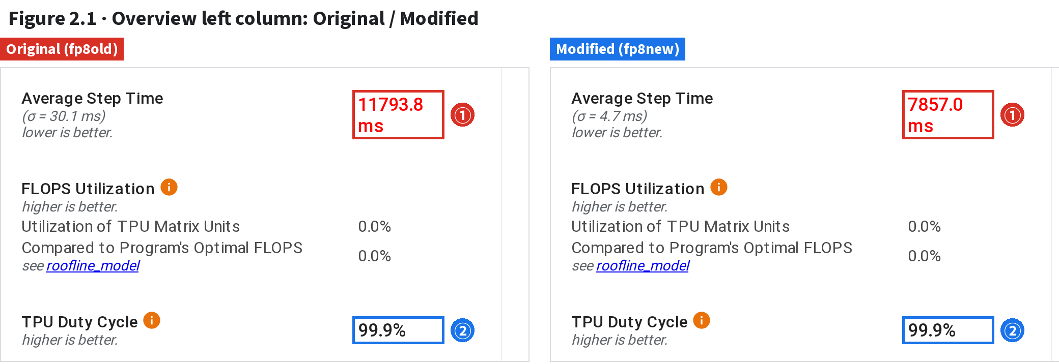
| # | What | On the page (boxes drawn at its text) |
|---|---|---|
| ① | Average Step Time | Original / Modified: 11,793.8 / 7,857.0 ms (XProf’s mean of 3 host-recorded steps; 0.2–0.3% above the median jit_train_step) |
| ② | TPU Duty Cycle | TensorCore busy share: 99.9% in both. Stalling on a done for communication counts as “busy”, so it only rules out long idle gaps |
A profile opens on Overview by default. Two questions: how long is a step, and does the TensorCore sit idle for long? Duty Cycle also counts stalling on a done for communication (2.5) as work, so it only rules out long idle stretches; the wait itself is in Trace Viewer. The rest of the column: 2.1B.
The lecture’s 7 profiles are public in GitHub Release topic07-hy3-profiles-v1 (Hy3 training on 64 TPU v7 chips; each is 3 steps from one host, 1.2–1.45 GB unpacked; only host names changed, to gke-node-N). Four copy-ready steps from download to first view:
# 1. Download (7 assets, 0.86 GB in total; for one or two runs, fetch only those)
mkdir -p ~/hy3-prof && cd ~/hy3-prof
B=https://github.com/yangwhale/gpu-tpu-pedia/releases/download/topic07-hy3-profiles-v1
for r in fp8old fp8new fp8nat r3anat fp8tk bf16old bf16new; do curl -fLO $B/hy3-$r.tar.zst; done
curl -fLO $B/SHA256SUMS && sha256sum -c SHA256SUMS
# fetched only some? add --ignore-missing; on macOS use shasum -a 256 -c SHA256SUMS
# 2. Unpack (9.2 GB in total): each tar already holds <run>/plugins/profile/<timestamp>/<host>.xplane.pb
# no zstd command? install it first: apt install zstd / brew install zstd
for f in hy3-*.tar.zst; do zstd -dc "$f" | tar -xf -; done
# 3. Install open-source XProf and point it at this directory
# ==2.23.1 is the version behind the screenshots; drop it for the latest
pip install xprof==2.23.1
xprof --logdir ~/hy3-prof --port 6311
# or use TensorBoard: pip install tensorboard tensorboard-plugin-profile
# then tensorboard --logdir ~/hy3-prof --port 6311 and open the PROFILE page
# 4. Open http://127.0.0.1:6311/ in a browser
# pick a run in the Sessions dropdown on the left (e.g. fp8old/2026_08_15_03_57_28), and a tool under Tools<logdir>/<run>/plugins/profile/<timestamp>/<host>.xplane.pb: each logdir subdirectory is one run. Unpacked, ~/hy3-prof holds 7 run directories; your own profiles laid out the same way appear alongside.| run | What | Median step (ms) | Unpacked file |
|---|---|---|---|
fp8old | FP8 original recipe (tokamax, injected tiles 512 / 2048 / 1536) | 11,758.2 | fp8old/plugins/profile/2026_08_15_03_57_28/gke-node-1.xplane.pb |
fp8new | FP8 modified recipe (native + 12 new tile values): 50% faster | 7,842.1 | fp8new/plugins/profile/2026_08_15_04_11_46/gke-node-1.xplane.pb |
fp8nat | rerun of fp8new | 7,846.1 | fp8nat/plugins/profile/2026_08_15_16_59_57/gke-node-4.xplane.pb |
r3anat | second rerun of fp8new | 7,840.1 | r3anat/plugins/profile/2026_08_16_01_29_28/gke-node-5.xplane.pb |
fp8tk | original recipe, no tiles injected (default 128×128×128): 375 s run | 375,160.0 | fp8tk/plugins/profile/2026_08_15_17_48_55/gke-node-4.xplane.pb |
bf16old | BF16 before the change (tokamax, injected tiles) | 21,747.2 | bf16old/plugins/profile/2026_08_15_09_13_02/gke-node-2.xplane.pb |
bf16new | BF16, after the same change (native + the same 12 tile values) | 20,693.8 | bf16new/plugins/profile/2026_08_15_09_28_25/gke-node-3.xplane.pb |
fp8old, modified fp8new; the other five appear in 3.5 (the 375 s run), Section 5 (BF16) and the exercises page. For your own profile, swap in its run name, timestamp, host and the windows below.http://127.0.0.1:6311/?run=fp8old/2026_08_15_03_57_28&tag=overview_page&host=gke-node-1, or pick Overview Page under Tools in the home page’s left column.view_start/view_end (ms from the profile start). These lines print the link; change run and window to open any screen in this lecture:import urllib.parse as u
D = {"fp8old": ("2026_08_15_03_57_28", "gke-node-1"),
"fp8new": ("2026_08_15_04_11_46", "gke-node-1"),
"fp8nat": ("2026_08_15_16_59_57", "gke-node-4"),
"r3anat": ("2026_08_16_01_29_28", "gke-node-5"),
"fp8tk": ("2026_08_15_17_48_55", "gke-node-4"),
"bf16old": ("2026_08_15_09_13_02", "gke-node-2"),
"bf16new": ("2026_08_15_09_28_25", "gke-node-3")}
run, vs, ve = "fp8old", 25476.963, 25512.640 # original recipe, forward, layer 40 (Figure 2.4A)
d, host = D[run]
data = f"/data/plugin/profile/data?run={run}/{d}&tag=trace_viewer@&host={host}&hosts={host}"
print("http://127.0.0.1:6311/data/plugin/profile/trace_viewer_index.html?is_streaming=true&is_oss=true"
f"&trace_data_url={u.quote(data, safe='')}&view_start={vs}&view_end={ve}")
/device:TPU:0 and its two SparseCores → Expand All. Trace Viewer opened from the home page’s Tools ignores the link’s window: you get the whole session.fp8old / fp8new, tool overview_page; read only the left column, Performance Summary.⭐ Of the 7 left-column cells in open-source 2.23.1’s Overview, two are worth reading: step time and Duty Cycle. FLOPS and HBM show 0.0%; Op Placement and Eager are fixed for JAX training; SparseCore step time and idle get no cell.
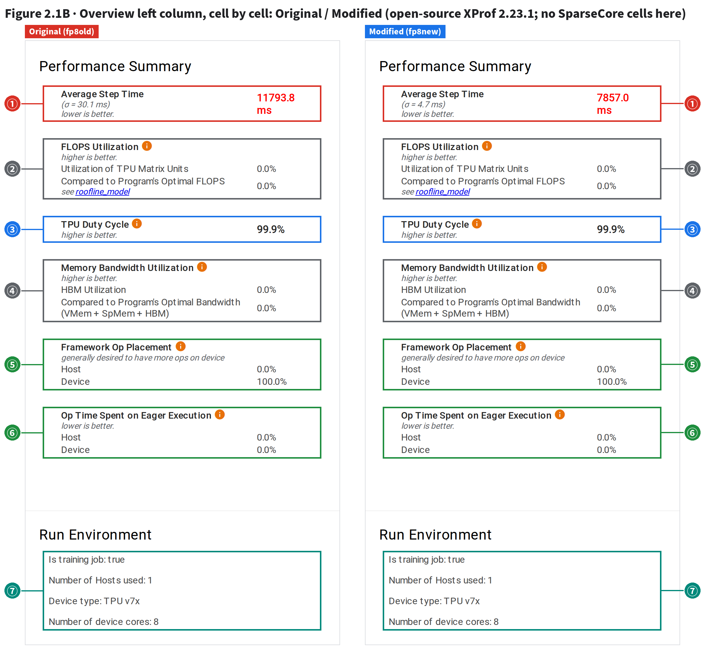
| # | What | Both readings (verbatim page text; extras in parentheses from the same page’s data endpoint) |
|---|---|---|
| ① | Average Step Time | 11,793.8 / 7,857.0 ms (σ 30.1 / 4.7 ms): 3-step mean, steps cut at host-recorded boundaries; 0.2–0.3% above §0.1’s median jit_train_step |
| ② | FLOPS Utilization ×2 | 0.0% in both: uncomputed in open-source 2.23.1, not really zero. Read utilization in Roofline and HLO Op Profile (Section 3) |
| ③ | TPU Duty Cycle | 99.9% / 99.9%: TensorCore busy share. Only 11.09 / 12.00 ms idle per step (data endpoint tc_idle_ms_average: the Step-time Graph’s TensorCore idle, right) |
| ④ | Memory Bandwidth Utilization ×2 | 0.0% in both: as ②, not computed by open-source XProf |
| ⑤ | Framework Op Placement | Host 0.0%, Device 100.0% (both): all ops on the device, as always in JAX training; no help here |
| ⑥ | Op Time Spent on Eager Execution | Host and Device 0.0%: nothing runs eagerly op by op (JAX jit-compiles the whole step); no help here |
| ⑦ | Run Environment | Training job, 1 host, TPU v7x, 8 device cores (4 chips × 2 TensorCores). Same in both |
2.1 read only ① and ③; first-timers ask whether the other five cells matter. Side by side, ② and ④ are 0.0% in both and ⑤ ⑥ ⑦ match word for word: only ① and ③ differ. Is the SparseCore busy? The column has no cell for it, and the Step-time Graph on the right plots only the TensorCore; its busy time and traffic are in its Trace Viewer row (2.4, 2.5).
The page’s data endpoint has these fields (command in “Open it yourself”):
| Field in the data endpoint | Meaning (from the field name) | Original | Modified |
|---|---|---|---|
sc_step_time_ms_average | SparseCore step time | 8,606.2 ms | 5,001.9 ms |
sc_idle_ms_average | SparseCore idle | 5,234.02 ms | 3,341.18 ms |
sc_compute_ms_average | SparseCore compute | 1,582.65 ms | 1,622.52 ms |
sc_infeed_ms_average | SparseCore infeed | 0.00 ms | 0.00 ms |
sc_outfeed_ms_average | SparseCore outfeed | 0.00 ms | 0.00 ms |
tc_idle_ms_average | TensorCore idle (for reference) | 11.09 ms | 12.00 ms |
xprof/convert/op_stats_to_input_pipeline_analysis.cc, each SparseCore’s compute per step = step time − idle. Within a step, step time and idle are averaged over the 16 SparseCores, but compute takes the minimum of the 16; then all are averaged over steps.
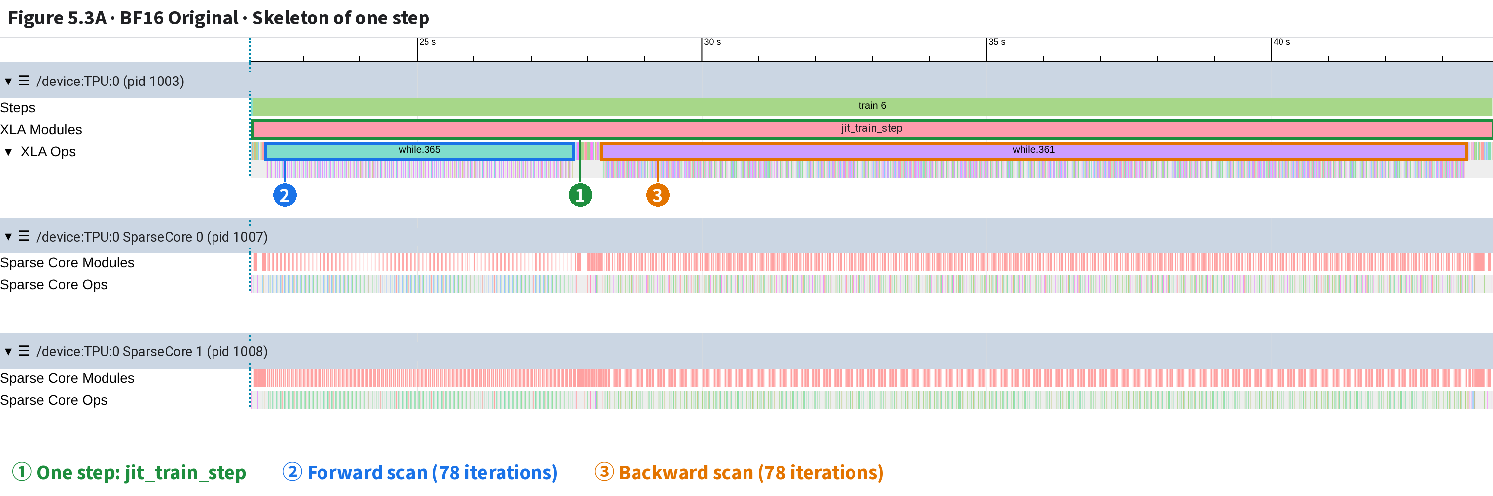
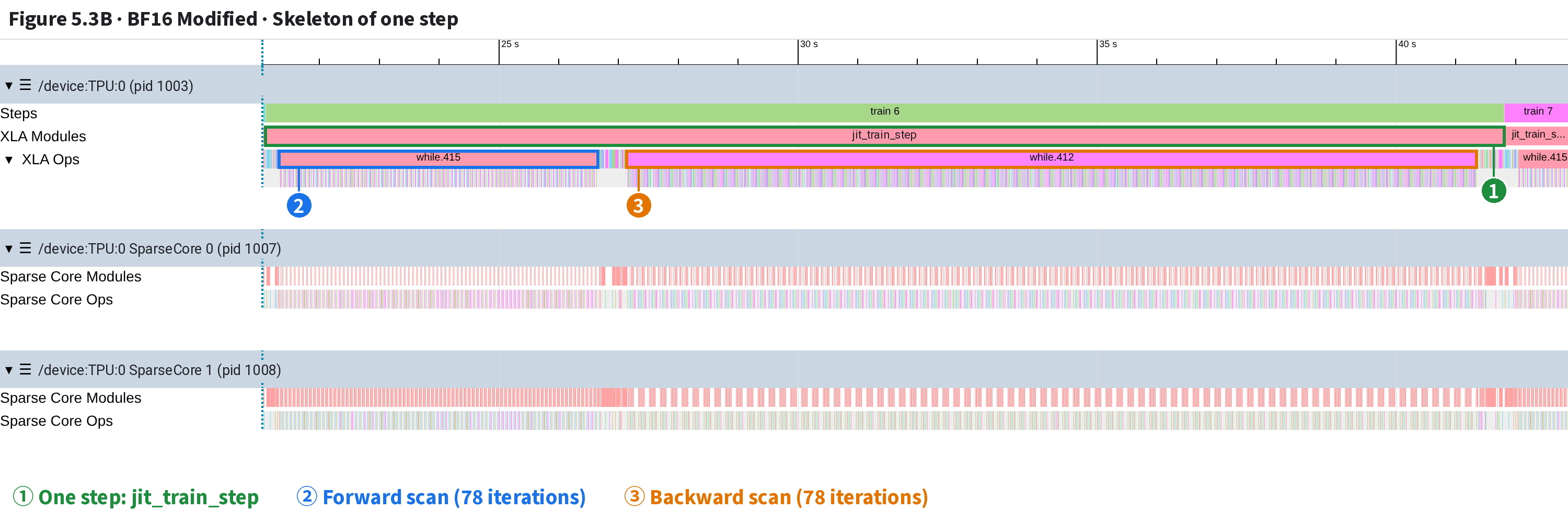
So step time − idle = 8,606.2 − 5,234.02 = 3,372.2 is the mean compute; sc_compute’s 1,582.65 is the idlest core’s. SparseCore steps follow its own Sparse Core Steps row, not TensorCore steps.tcIdleTimeMs): Original 5.5 / 13.9 / 13.9 ms, Modified 5.8 / 15.3 / 15.0 ms. Step 0 is just over 5 ms in both runs, the next two in the teens [cause not checked].fp8old / fp8new, tool overview_page: http://127.0.0.1:6311/?run=fp8old/2026_08_15_03_57_28&tag=overview_page&host=gke-node-1; the left column reads ①→⑦ from top to bottom (scroll down for Run Environment).sc_* fields the page doesn’t show): curl -s --compressed "http://127.0.0.1:6311/data/plugin/profile/data?run=fp8old/2026_08_15_03_57_28&tag=overview_page&host=gke-node-1" | python3 -m json.tool | grep -E "sc_|tc_idle"; change the run name and timestamp to read the modified run.⭐ One step per screen: a forward loop and a backward loop, 78 iterations each, one layer per iteration. Both runs share this skeleton; the modified one is a third shorter.
Trace Viewer draws each op as a slice on a time axis and opens on the whole session, dozens of rows (recording stop 3). Four moves: Collapse All → close the rest (X at the right end), keeping only
/device:TPU:0 and its SparseCore 0 and SparseCore 1 (other devices look the same)
→ Expand All → on XLA Modules, click the median step’s jit_train_step and press f to fill the screen.
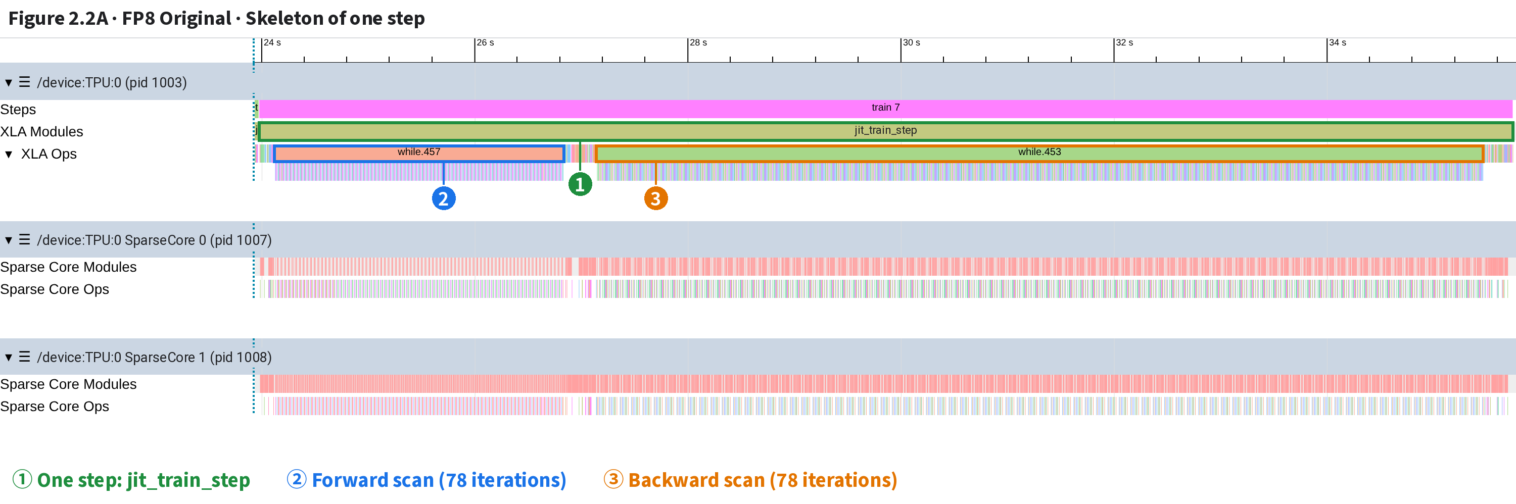
| # | What | How to tell (names, times from the xplane) |
|---|---|---|
| ① | One step: jit_train_step | jit_train_step on the XLA Modules row, 11,758.17 ms (median of 3 complete steps) |
| ② | Forward scan (78 iterations) | while.457, 2,704.03 ms, 78 iterations (the compiler peels layer 0 off before the loop and runs it separately; fold below) |
| ③ | Backward scan (78 iterations) | while.453, 8,313.25 ms, 78 iterations, layers counting down |
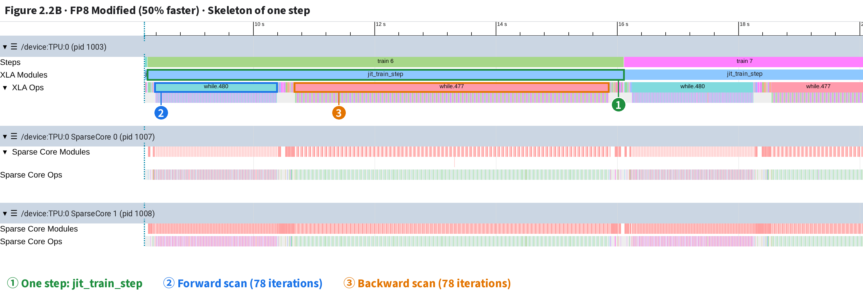
| # | What | How to tell (names, times from the xplane) |
|---|---|---|
| ① | One step: jit_train_step | jit_train_step on the XLA Modules row, 7,842.07 ms (median of 3 complete steps) |
| ② | Forward scan (78 iterations) | while.480, 1,998.05 ms, 78 iterations (the compiler peels layer 0 off before the loop and runs it separately; fold below) |
| ③ | Backward scan (78 iterations) | while.477, 5,168.26 ms, 78 iterations, layers counting down |
A v7 chip has 2 TensorCores, which the profile counts as 2 devices; keeping one is enough.
scan: with scan_layers=True in the config, MaxText compiles the 79 structurally identical MoE layers into one while loop, one layer per iteration; on the trace it is the two big blocks ② ③.
Forward 2,704.0 → 1,998.1 ms, backward 8,313.2 → 5,168.3 ms. Both shrink, the backward far more (by 3.1 s).
📌 Step bounds: the median jit_train_step on TPU:0 XLA Modules (median of 3 complete steps), fp8old 23,983.849–35,742.021 ms, fp8new 8,262.067–16,104.132 ms (from profile start).
📌 Bounds of the two whiles: fp8old while.457 24,125.829–26,829.855, while.453 27,147.384–35,460.634; fp8new while.480 8,386.321–10,384.372, while.477 10,687.259–15,855.523 ms. The five parts sum to the step time within 0.1 ms.
📌 What each part holds, told by top-level leaf names, tf_op and shapes: fusion.502 before the loops reads the vocabulary (bf16[120832,4096]); the dense layer’s intermediate dim is 13,312 (config mlp_dim); between the loops are two bf16[7,4096,120832] output-head matmuls and 8 expert matmuls (gmm 3, gmm_t 3, tgmm 2) of the MTP layer; the multiply_reduce_fusion after the backward loop holds AdamW’s first and second moments and weight decay (0.9 / 0.95 / 1e-8 / 0.1, matching the config).
📌 Why MoE layer 0 is outside the loops: the compiler peeled it off the scan, forward before, backward after (sources in the main-text fold “Why 79 layers loop only 78 times”).
| Stop | Action | What you see |
|---|---|---|
| 1 | The window in the link opens the original recipe’s forward layer 40, already tidied to TPU:0 + two SparseCores | 35.7 ms on screen |
| 2 | Hover over gmm_megablox.16, press W 3 times | Zooms around the mouse to 10.6 ms on screen; the name appears |
| 3 | Press S 3 times to zoom back, D 2 times to pan right | Window moves right by about 10 ms; A pans left |
| 4 | A to come back, click gmm_megablox.16 | Details: Wall Duration 3,425,196 ns (drop the last 6 digits to read ms) |
| 5 | Click all-gather.575 on the SparseCore, press m | Interval marked on the ruler (3.981 ms); over the same span the TensorCore computes gmm_megablox.16 |
| 6 | With it still selected, press f | The slice fills the screen; the 3.981 ms marked by m is exactly one screen wide |
| 7 | Same layer in a new page: click one, hold Ctrl (Command on a Mac) and click two more | “3 items selected.”, Totals 10,106,678 ns = 10.1 ms for all three |
| 8 | Type gmm_megablox.16 into Find Events at the top, press Enter | “0 of 1872”, view doesn’t move; 1,872 = 78 iterations × 3 steps × 8 TensorCores, closed processes included. Gotcha: closed processes all come back |
| 9 | Click the → right of the box | Jumps to the first match, the one in train 5: 3,329,133 ns |
Shortcuts need the mouse over the timeline; durations are in ns; clicks while loading don’t count. Full video: topic07-xrec-basics.en.mp4.
⭐ Only two rows are measured: XLA Ops (TensorCore) and Sparse Core Ops (SparseCore), where a slice = one instruction run once. The other rows are labels.
| Row | What it is | What to read |
|---|---|---|
Steps | Training step (train 5/6/7), host-logged | Label: find the step; not timed |
XLA Modules | Compiled program running; one jit_train_step = one step | A step’s start and end |
XLA Ops (measured) | Every TensorCore instruction: big loop slices on top, their instructions below | Time ops on the bottom level only |
Sparse Core Modules | Program running on the SparseCore | Label |
Sparse Core Ops (measured) | Every SparseCore instruction: collectives (all-gather, reduce-scatter, all-reduce) and per-expert token moves (gather_offload) | Communication time |
Collectives run on the SparseCore here: the TensorCore issues one and keeps computing while the SparseCore moves data. So to see if communication shrank, check the SparseCore row; the TensorCore keeps only start (issue) and done (wait), as in the small 2.5 example.
📌 Every event on the right is from the fp8old xplane (TPU:0’s XLA Ops; Sparse Core Ops on both SparseCores), the same data as the static figure and agdone animation in §2.5: start 31,219.512 ms; all-gather.547 on SparseCore 0, 31,223.777–31,226.183 ms (2.406 ms); TensorCore all-gather.548.cloned.1.call-done, 31,225.002–31,226.183 ms (1.181 ms); after release, gmm_megablox.14 starts at 31,226.184 ms.
📌 The small cluster right after start on the TensorCore is a few dozen tiny slices within a dozen or so µs (sort, slice, copy, etc.), not drawn individually. The slices on SparseCores 0 and 1 are gather_offload_custom_fusion.68/.64 (per-expert token moves).
📌 Row names come from Trace Viewer in our local open-source XProf 2.23.1. Framework Name Scope is really several rows (one per name-path segment), merged into one here. The xplane also has an Async XLA Ops row, not used in the text, so not drawn.
Click a slice for Details below: fields on the left, links and up/downstream on the right. We try a compute op and a collective done.
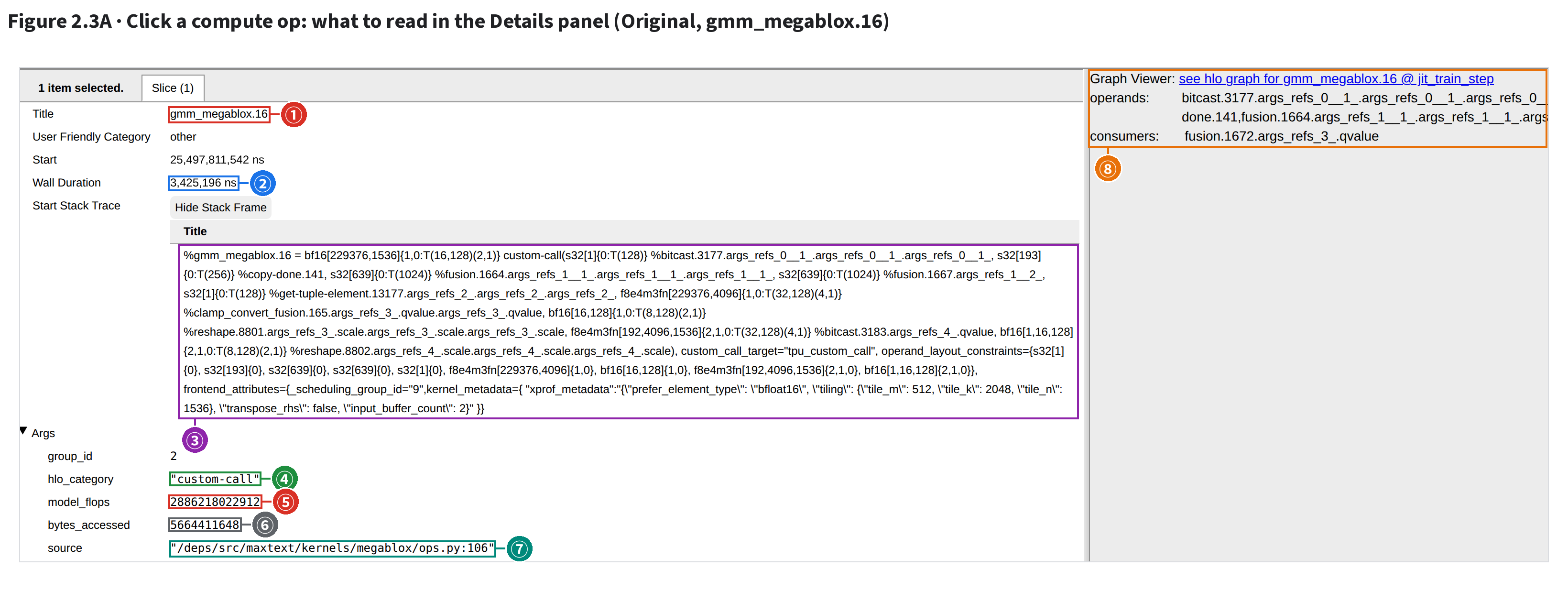
| # | What | What to read (boxes mark where the text sits) |
|---|---|---|
| ① | Title: slice name | gmm_megablox.16: its name in the HLO (minus the %) |
| ② | Wall Duration: how long | 3,425,196 ns = 3.43 ms: the slice’s width, in ns. The Start line above is the time since profile start |
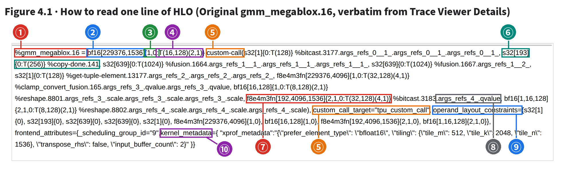
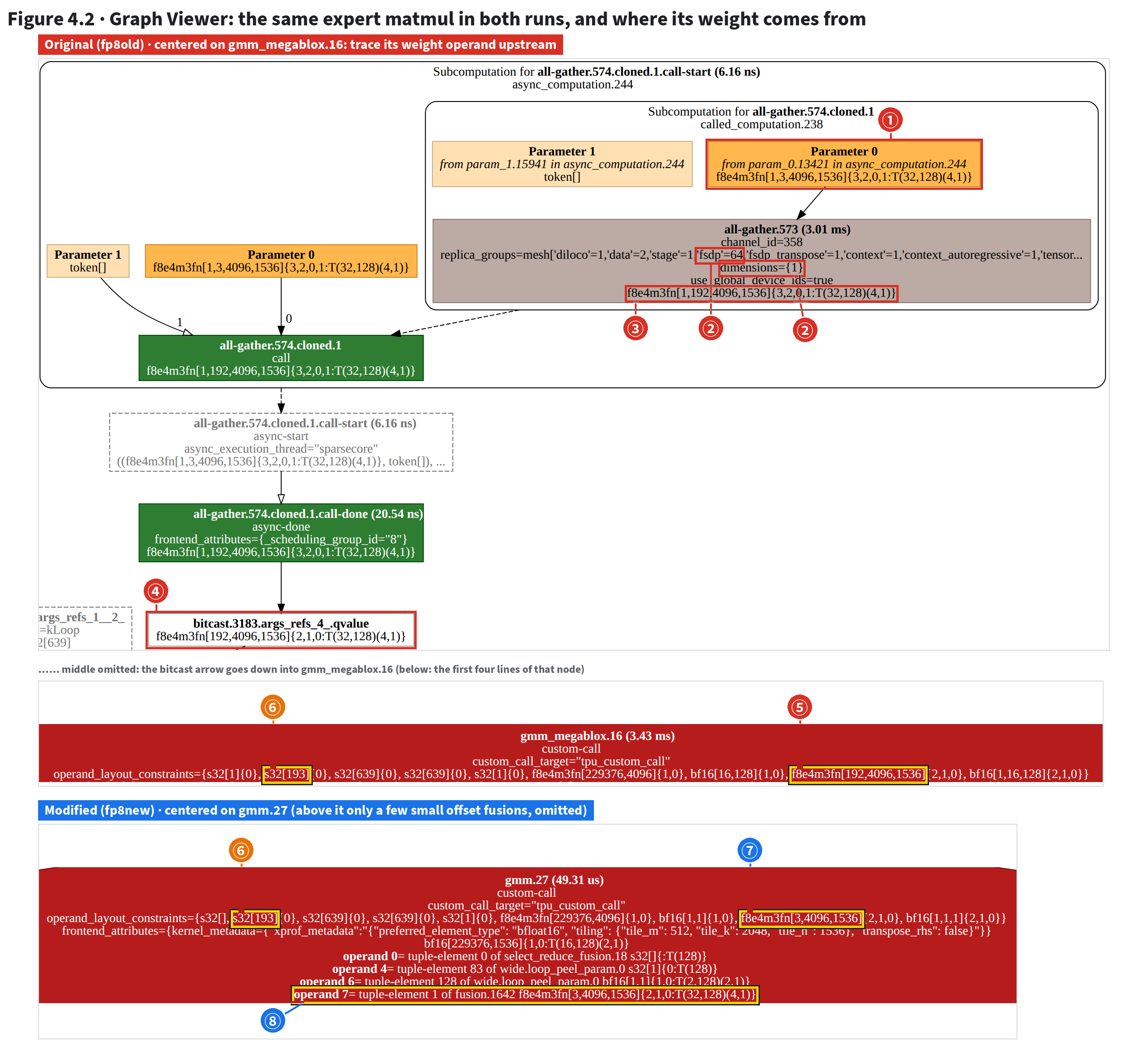
| ③ | Start Stack Trace: the HLO text | The compiled line: output shape plus each operand’s type and name. Section 4 counts shapes from it (Figure 4.1 reads it symbol by symbol) |
| ④ | hlo_category: which category | "custom-call": a call to an external kernel (here the Pallas expert matmul). Section 3’s Op Profile groups categories by this field |
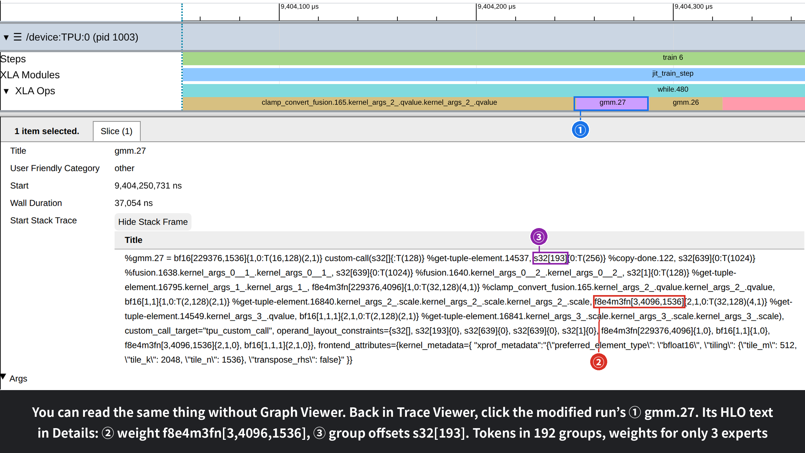
| ⑤ | model_flops: FLOPs booked | 2,886,218,022,912 = 2 × 229,376 × 4,096 × 1,536: computed from the shapes. The modified recipe’s gmm.27 runs only 0.04 ms yet shows the same number (we checked it locally); the 117% in §3.2 comes from this booking |
| ⑥ | bytes_accessed: bytes booked | 5,664,411,648: the compile-time estimate of bytes read and written, also from the shapes (modified recipe’s gmm.27: 5,664,407,552, almost unchanged) |
| ⑦ | source: which Python line | megablox/ops.py:106: the return gmm_fwd_bwd(…) line in public MaxText (gmm’s entry point). The source_stack below is the full call stack, which §4.5 follows back to the code |
| ⑧ | Right column: links, up/downstream | The Graph Viewer link (§4.3 enters here); operands: whose outputs it reads; consumers: who uses its output |
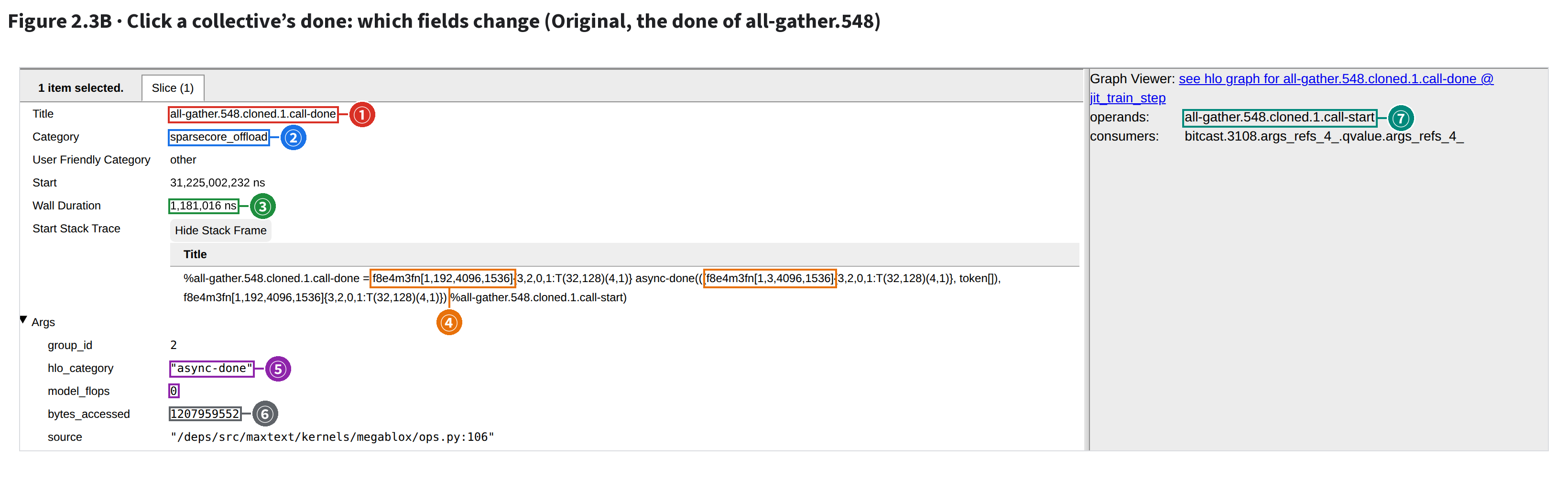
| # | What | What to read (boxes mark where the text sits) |
|---|---|---|
| ① | Title: …call-done | all-gather.548.cloned.1.call-done: a collective splits into two instructions, issue (start) and wait for completion (done); this is the done, the subject of the 2.5 example |
| ② | Category: sparsecore_offload | This collective is handed to the SparseCore; compute ops lack this line |
| ③ | Wall Duration: how long the TensorCore waited | 1,181,016 ns = 1.18 ms: how long the TensorCore waits on done for the SparseCore to finish, i.e. this collective’s exposed part |
| ④ | HLO: what is moved | Result f8e4m3fn[1,192,4096,1536], input [1,3,4096,1536]: each device gathers its own 3 experts’ FP8 weights into all 192 |
| ⑤ | hlo_category + model_flops | "async-done", 0: nothing booked, just waiting |
| ⑥ | bytes_accessed: bytes moved | 1,207,959,552 = 192 × 4,096 × 1,536 × 1 byte: the FP8 weights of 192 experts, about 1.21 GB |
| ⑦ | operands: the paired start | all-gather.548.cloned.1.call-start: its issuing instruction; Find it by name in Trace Viewer |
model_flops / bytes_accessed are booked at compile time from the shapes, not measured: they ignore how many rows the kernel actually computed. Only Wall Duration is measured.fp8old view_start=25476.963, view_end=25512.640 ↗ Open; click gmm_megablox.16 on the TensorCore (the same one as stop 4 of the basics recording); scroll down to Args at the bottom of Details.fp8old view_start=31222.3, view_end=31227.3 ↗ Open (backward layer 40, the 2.5 window); click all-gather.548.cloned.1.call-done, the slice in the middle of the TensorCore’s second XLA Ops level.| Name | How to read it |
|---|---|
all-gather.548.cloned.1.call-done | all-gather is the operation, .548 the instruction’s number in the program (a different number is a different instruction). Middle suffixes like .cloned.1 come from compiler cloning or rewriting; skip them [inferred from the naming pattern]. Trailing call-start/call-done are one async run’s issue and wait. The SparseCore slice doing the move is 1 lower (all-gather.547, 2.5) |
gmm_megablox_transpose_rhs.10, gmm.27, splash_mha_fwd… | Pallas kernels: a self-chosen name (expert matmul, attention) plus a number. Same-named slices are one kernel called many times |
gather_offload_custom_fusion.68, gather_offload_async_done.6 | Per-expert token moves offloaded to the SparseCore: the first runs there, the second is the TensorCore waiting for it |
broadcast_select_fusion, select_add_fusion, clamp_convert_fusion | When XLA fuses elementwise ops, the name lists them [inferred from the naming pattern]: clamp_convert is FP8 quantization (clamp, then cast); select picks one of two by condition |
fusion.1176{1} (in Memory Viewer) | The number in braces is which of the instruction’s outputs this is: one instruction can produce several buffers |
⭐ Zoom to a few ms around a kernel and expand all rows under TPU:0: a column stacks a dozen-plus slices. Which level holds the duration? Is each level nested in the one above, or independent?
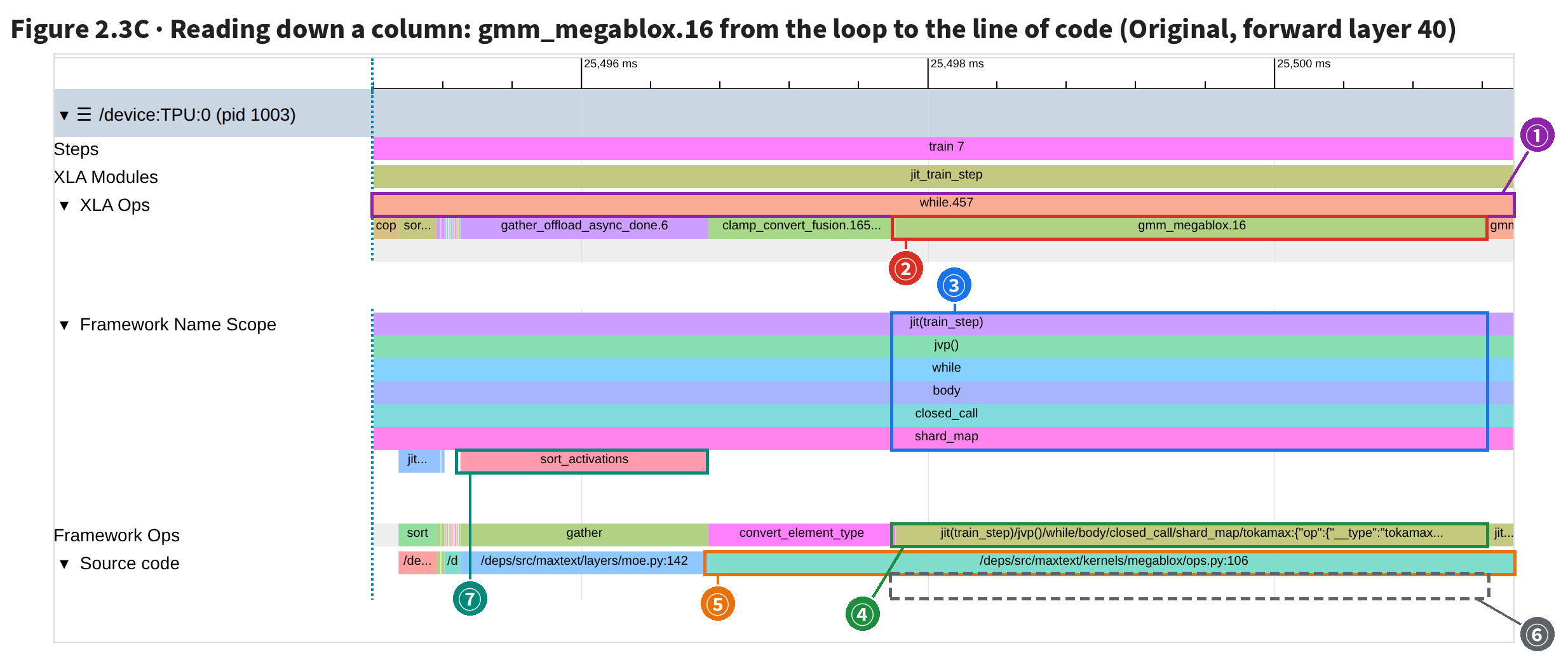
| # | What | How to tell (boxes from xplane event times and DOM rows) |
|---|---|---|
| ① | Top level: while.457 | The forward main loop: from 24,125.829, 2,704.03 ms, 78 iterations, one layer each. This screen spans only 6.6 ms, so the loop runs in from the left and out the right; neither end is visible. A container: the level below lies within its span |
| ② | Next level: leaf op gmm_megablox.16 | From 25,497.811 ms, 3.425 ms, nothing below: only a slice with nothing under it is one instruction executing once (a leaf). Time only this level: while.457’s 2,704 ms already includes it, so adding both double-counts |
| ③ | Framework Name Scope: the name path | jit(train_step) → jvp() → while → body → closed_call → shard_map: the leaf’s tf_op split into a path, one segment per row, outer around inner. jvp() = forward (backward: transpose(jvp())), while/body = scan loop body, shard_map = per-device part. No iteration (layer) index |
| ④ | Framework Ops: the leaf’s tf_op | The full tf_op string: the first half is ③’s path; the trailing tokamax:{…} is the kernel name and config (the Pallas expert matmul). Left neighbors show only op names like gather, convert_element_type |
| ⑤ | Source code, upper: which Python line | /deps/src/maxtext/kernels/megablox/ops.py:106: the leaf’s Details source (innermost source-stack frame). Adjacent leaves from the same line merge into one, so it’s wider than ②: from clamp_convert_fusion.165 (FP8 quantization) past gmm_megablox.17 and off screen. The quantization happens in gmm’s entry point |
| ⑥ | Source code, lower: empty here | Source code stacks by time too: a container with a source takes the upper row, its leaves the lower (like the three small whiles in Figure 2.3D). while.457 has no source or tf_op, so ③④⑤ lack its level and the lower row here is empty |
| ⑦ | Left neighbor’s extra level: sort_activations | gather_offload_async_done.6 (1.43 ms) has an extra path segment, sort_activations; Source code: /deps/src/maxtext/layers/moe.py:142, the MoE step that sorts tokens by expert. A run of slivers usually belongs to one module; read down the column to see it. |
⭐ Stacked = contained: XLA Ops is a single row of events in the profile; XProf stacks it into two levels by which time range encloses which. Time only the bottom slice, a leaf op: nothing under it, one instruction run once.
The container above (here the forward loop while.457) already spans all its leaves. The bottom three rows are the leaf’s name path, tf_op (JAX’s tag for the op and its code) and code line, not more nesting.
Same for ⑦: its extra segment sort_activations and line maxtext/layers/moe.py:142
put the left neighbor gather_offload_async_done.6 in the MoE step sorting tokens by expert. Tiny slices nearby often share a module; read down a column.
Most HLO instructions run on the hardware as one block: a fusion compiles to one kernel, and the sub-computations of sort or reduce (just rules for comparing or adding two values) go into that same kernel.
Only while runs its body iteration by iteration at runtime; each body instruction logs an event, so they stack beneath it as sub-levels. JAX’s lax.scan, fori_loop and while_loop
all compile to while, as do library functions that use scan inside. A Python for unrolls at compile time: no while.
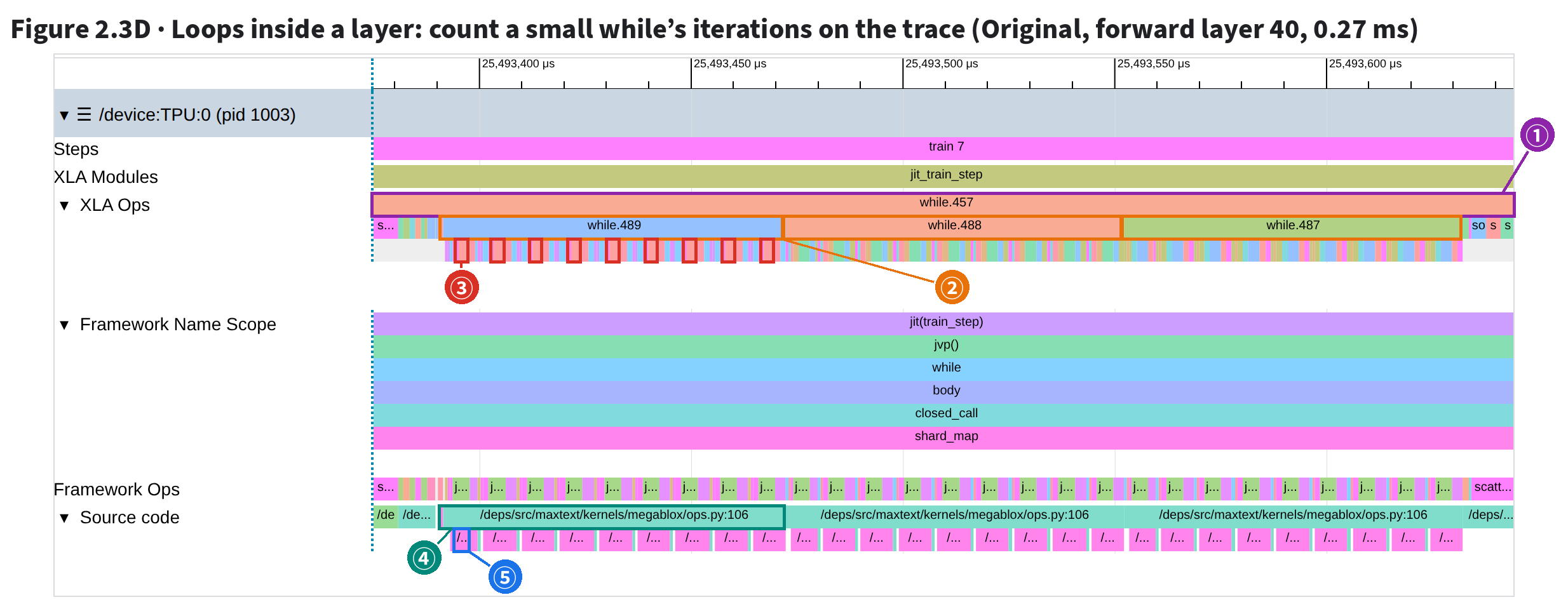
| # | What | How to tell (boxes from xplane event times and DOM rows) |
|---|---|---|
| ① | Level 1: while.457 | Forward main loop: the first slice beneath it, prepare_start_all-gather.570…, appears 78 times inside it = 78 iterations (forward layers 1–78); backward while.453 counts to 78 the same way |
| ② | Level 2: three small whiles | while.489/488/487, about 80 µs each, back to back just before the three expert matmuls: level-2 containers, not leaf ops |
| ③ | Level 3: loop body, once per iteration | Count any slice of the sub-level: the boxes mark the easy-to-spot gather_fusion.22, 9 times under while.489 (9 boxes); the first slice, copy.2136, also appears 9 times. The loop body repeats once per iteration → 9 iterations. All 936 small whiles in this step run 9 iterations, with 72 leaf ops each |
| ④ | Source code, upper: the container’s | megablox/ops.py:106: the small while’s own source, same start and end as ②, in the upper row |
| ⑤ | Source code, lower: each leaf’s | Read a leaf’s origin here; the slice above only says which line the whole while came from |
gather_fusion.22). The first, copy.2136, appears 9 times under while.489 = 9 iterations.
By the same count, forward while.457 and backward while.453 both run 78.op_name in the compiled HLO is jit(_searchsorted_scan_impl), inside the Tokamax expert matmul’s entry point: the jnp.searchsorted that finds each token’s position by expert.
By default it binary-searches with scan, in ⌈log₂(n+1)⌉ iterations (JAX source jax/_src/numpy/hijax.py). This while’s state holds an f32[449];
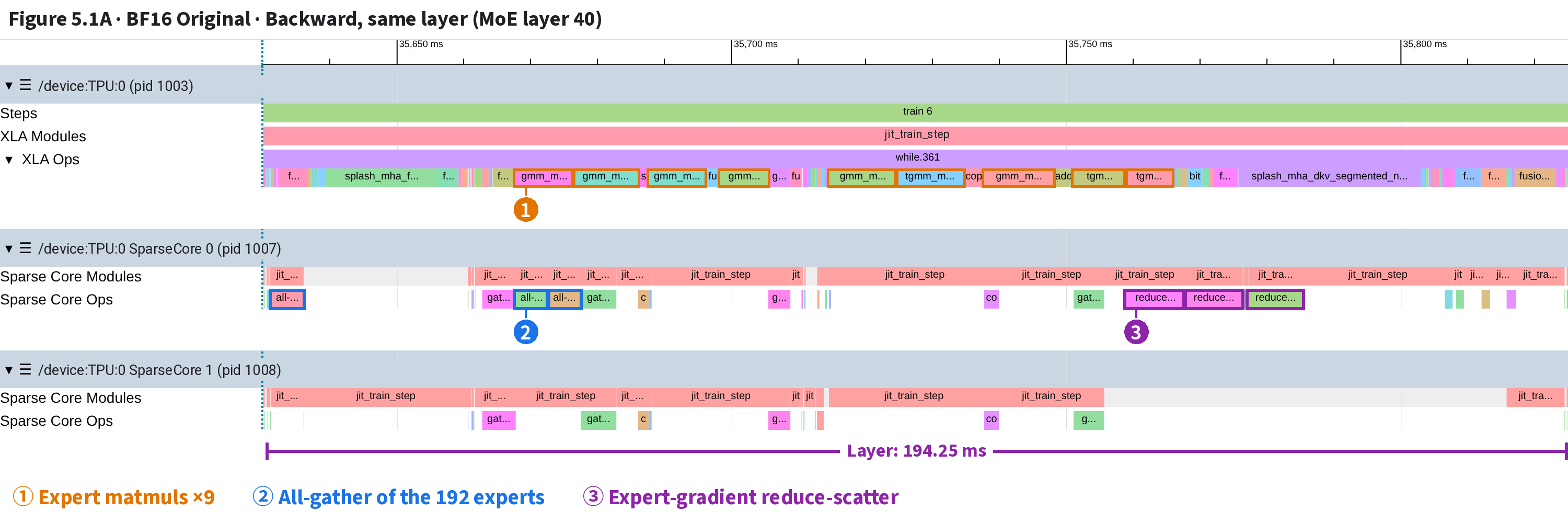
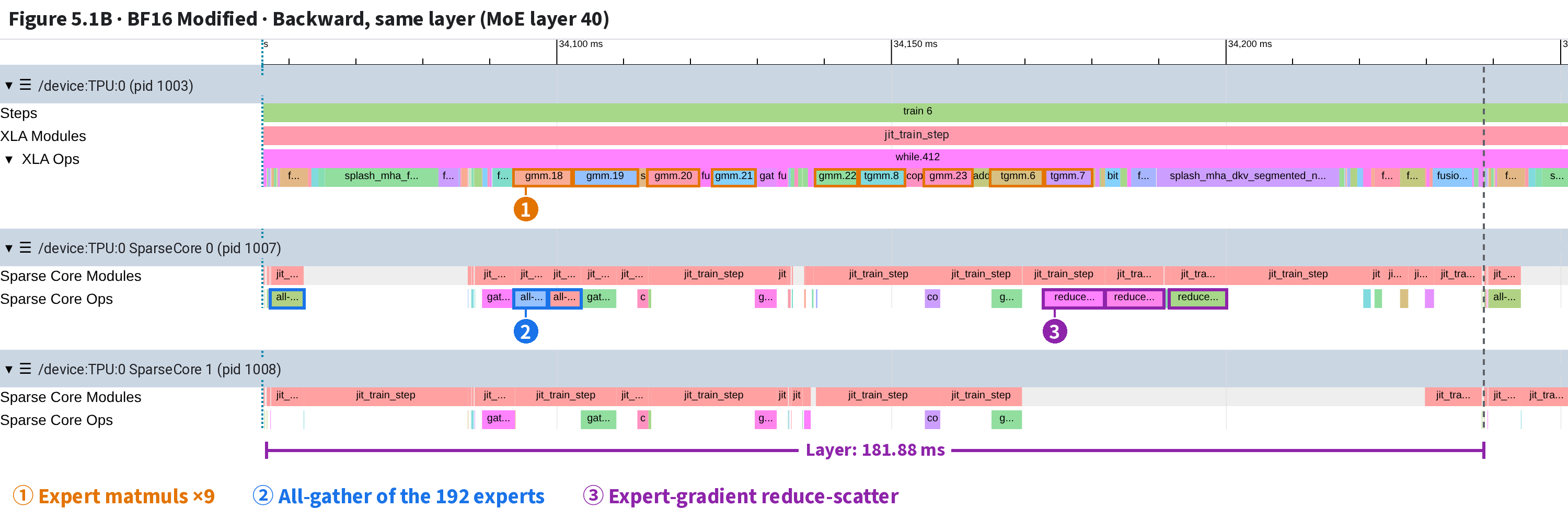
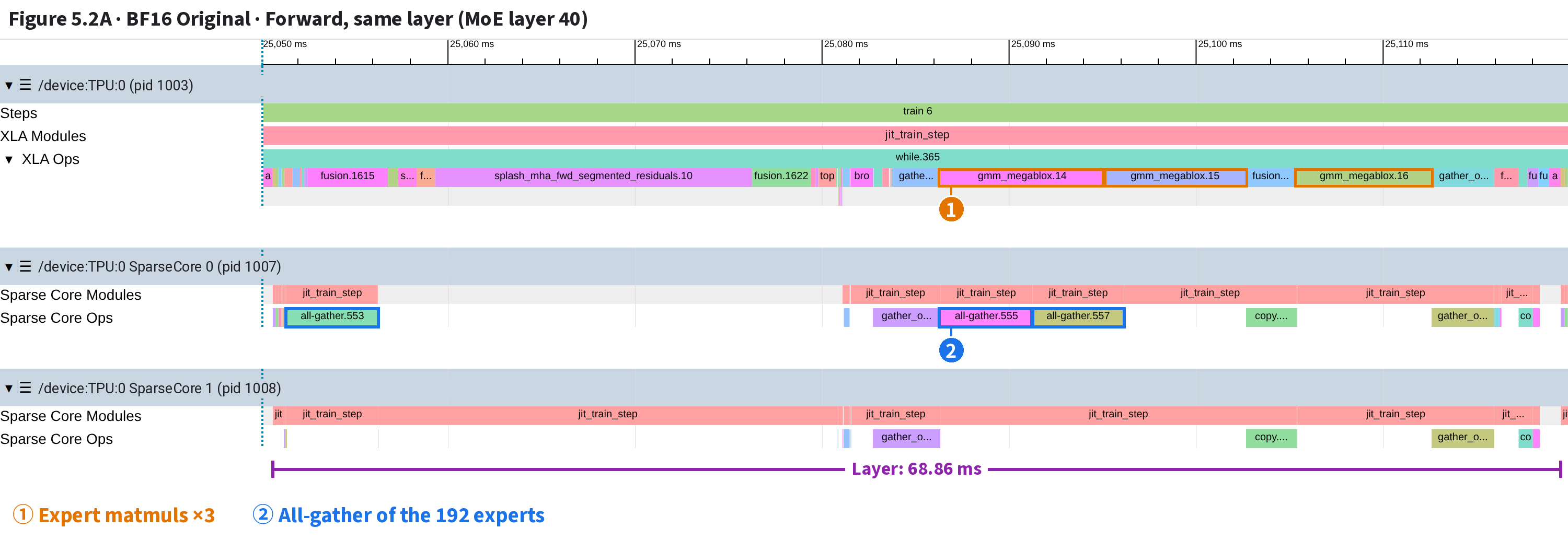
n = 449 gives exactly 9, matching the count on the trace [inferred: this f32[449] is the array being searched].source takes the upper row (④), its leaves’ the lower (⑤), so read a leaf’s origin from the lower row only. while.457 has no source or tf_op, so its column’s lower row is empty (⑥ in Figure 2.3C).fp8old, view_start=25,494.800, view_end=25,501.400. Expand All opens the Framework Name Scope, Framework Ops and Source code rows under TPU:0; click gmm_megablox.16 and check tf_op and source in Details.fp8old, view_start=25,493.375, view_end=25,493.645 (0.27 ms; names show as ga; click for full names).⭐ In modified layer 40 the SparseCore’s all-gather of the 192 experts is gone, as is the backward expert-gradient reduce-scatter. The expert matmuls shrink from 10.1 to 0.1 ms.
A whole step (11.76 s) is too wide for op names; zoom to one layer (tens of ms). Zooming 300-odd× with W from a full step drifts; a window written into the link is most reliable (see Open it yourself).
Both runs show layer 40 at the same window width, each left-aligned to the layer’s start.
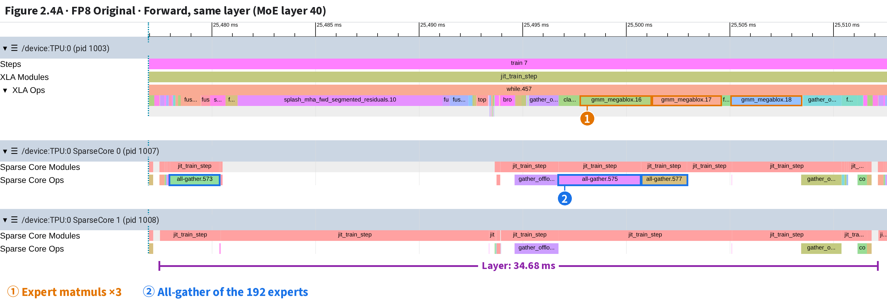
| # | What | How to tell (names and times from the xplane) |
|---|---|---|
| ① | Expert matmuls ×3 | TC: the layer’s 3 expert matmuls (gmm) total 10.11 ms: 3.43/3.33/3.35 ms Two boxes in the main image: gmm_megablox.16 + gmm_megablox.17 (from 25,497.812 ms, 3.425/3.328 ms); gmm_megablox.18 (from 25,505.087 ms, 3.354 ms) |
| ② | All-gather of the 192 experts | SC0: all-gathers 573/575/577 of the 192 experts’ weights, 2.38/3.98/2.21 ms; shapes like f8e4m3fn[1,192,4096,1536] Two boxes in the main image: all-gather.573 (from 25,477.978 ms, 2.380 ms); all-gather.575 + all-gather.577 (from 25,496.737 ms, 3.981/2.209 ms) |
| Bracket | Layer: 34.68 ms | Window = this layer plus 0.5 ms each side; the modified image has the same width, left-aligned to its own layer |
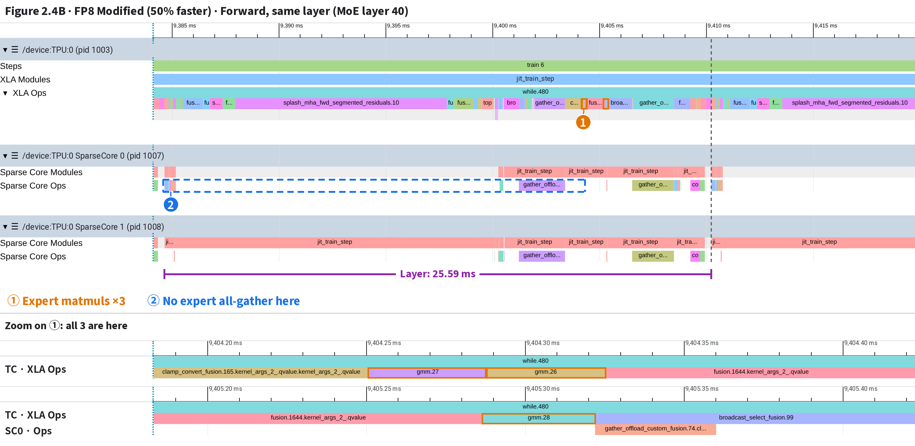
| # | What | How to tell (names and times from the xplane) |
|---|---|---|
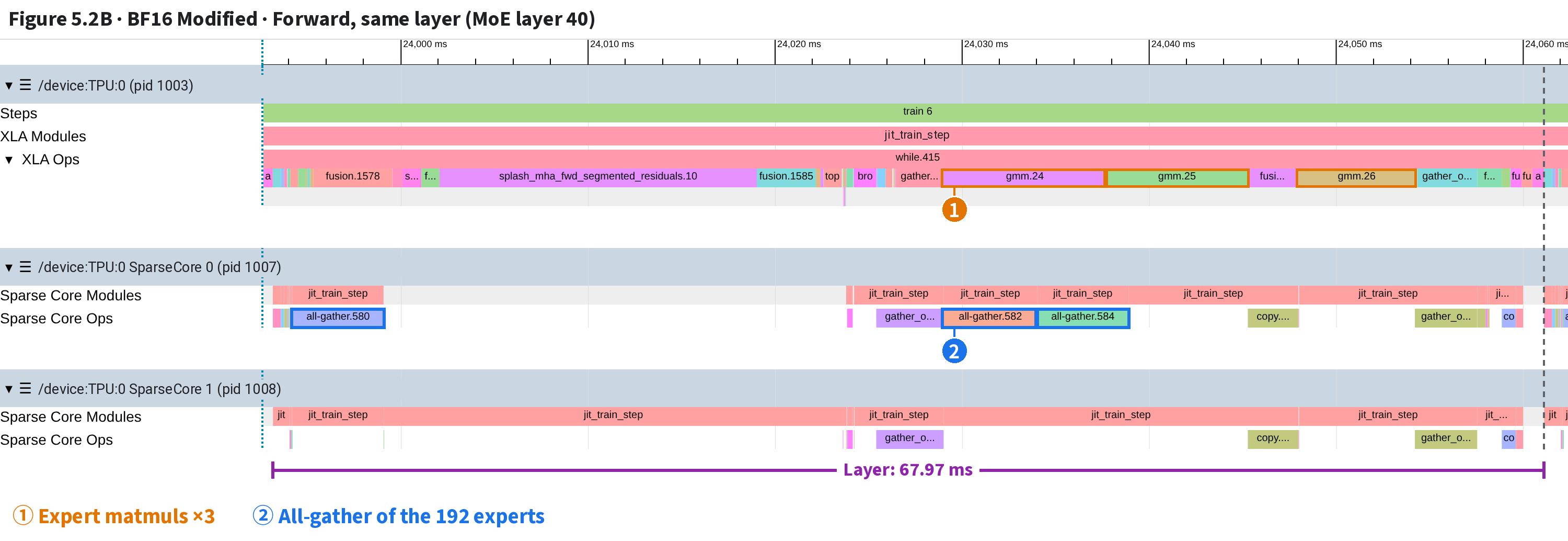
| ① | Expert matmuls ×3 | TC: the layer’s 3 expert matmuls (gmm) total 0.11 ms: 0.04/0.04/0.04 ms; boxes a few pixels wide (original, same layer: 10.11 ms) Two boxes in the main image: gmm.27 + gmm.26 (from 9,404.251 ms, 0.037/0.037 ms); gmm.28 (from 9,405.287 ms, 0.035 ms) |
| ② | No expert all-gather here | Dashed: layer start to the first gmm, the original’s ② slot. Here SC0 has no expert-weight all-gather, only 5 other small all-gathers (none the full [1,192,…] expert set, each ≤0.18 ms) and gather_offload (gathering tokens by route) |
| Zoom 1 | Window 9,404.18–9,404.42 ms | gmm.27 (0.037 ms), gmm.26 (0.037 ms); SC0 has no events in this span, so its row is absent |
| Zoom 2 | Window 9,405.18–9,405.42 ms | gmm.28 (0.035 ms) |
| Bracket | Layer: 25.59 ms | Gray dashed line: end of this layer; to its right is the next layer (A and B share one window width = the original’s layer) |
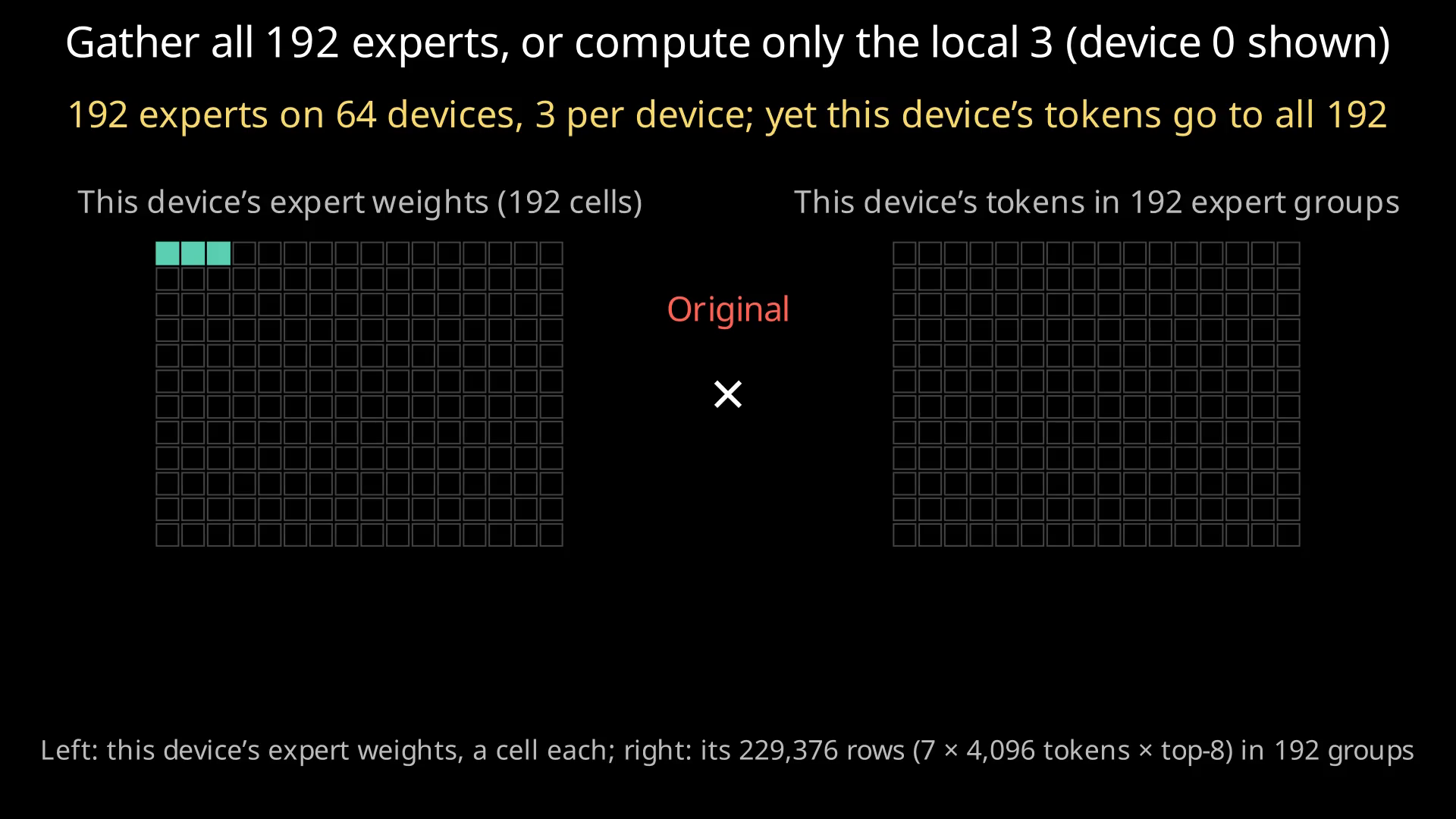
What all-gather does here: each device stores only 1/64 of the 192 experts and, when needed, gathers all of them from the 64 devices in the FSDP group. The original’s three are shaped like f8e4m3fn[1,192,4096,1536]: the leading 192 = all 192 experts.
In the modified run that stretch is empty but for a few tiny all-gathers (none covering the 192 experts) and gather_offload moving tokens per expert.
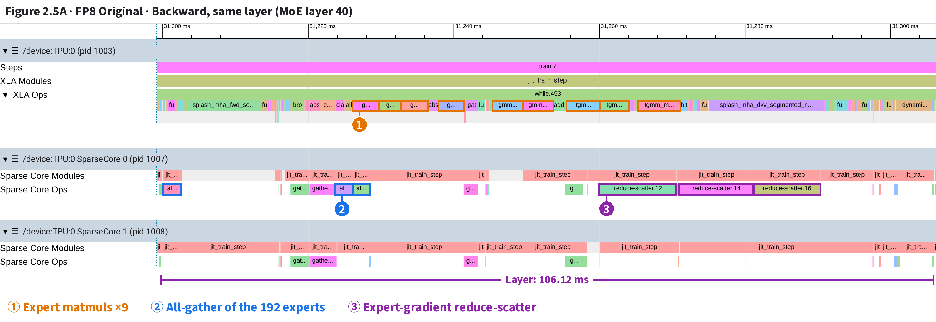
| # | What | How to tell (names and times from the xplane) |
|---|---|---|
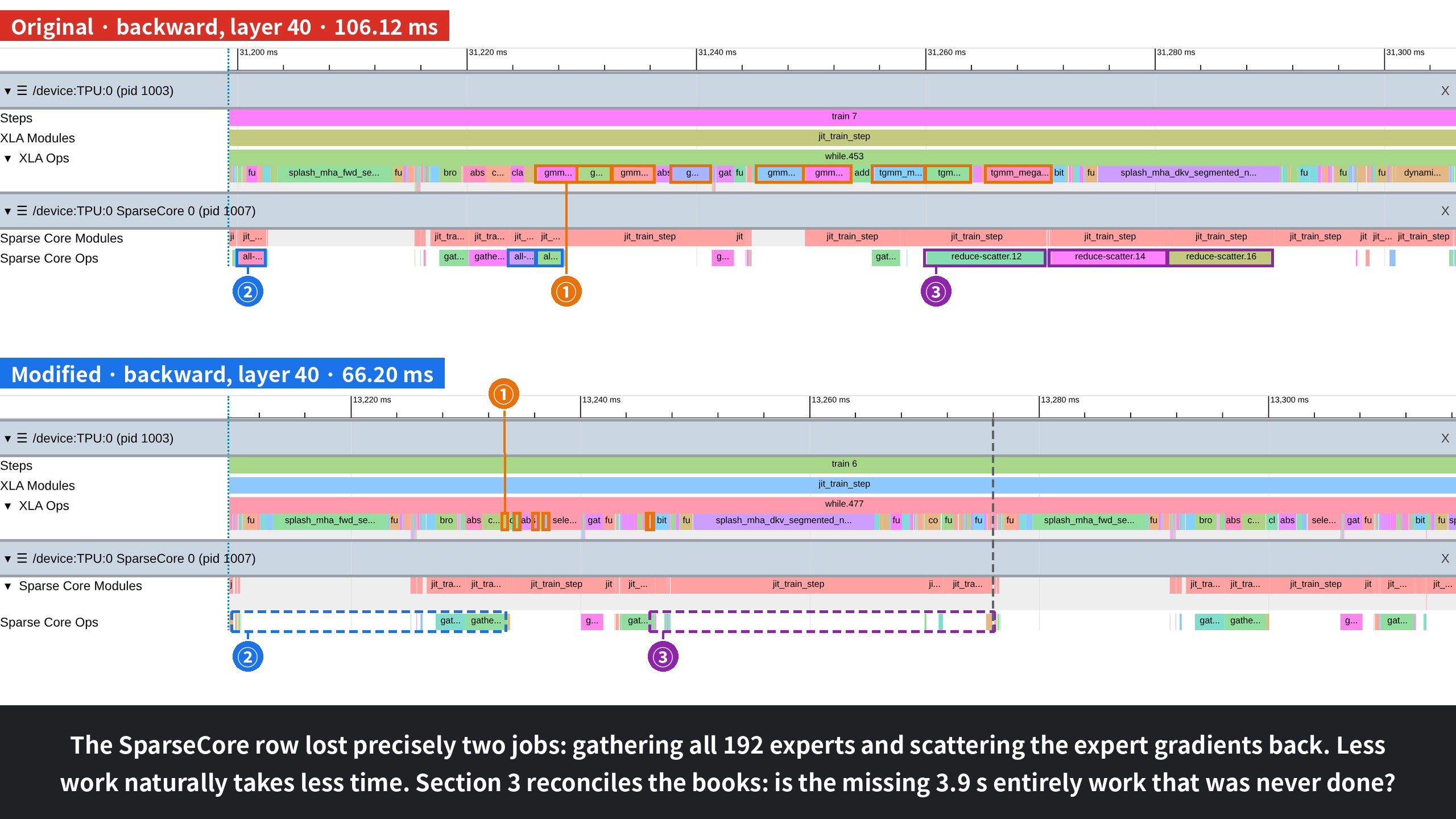
| ① | Expert matmuls ×9 | TC: the layer’s 9 expert matmuls (gmm/tgmm) total 35.69 ms Five boxes in the main image: gmm_megablox.14 + gmm_megablox.13 + gmm_megablox_transpose_rhs.10 (from 31,226.184 ms, 3.530/2.982/3.631 ms); gmm_megablox.15 (from 31,237.982 ms, 3.357 ms); gmm_megablox_transpose_rhs.12 + gmm_megablox_transpose_rhs.11 (from 31,245.398 ms, 4.050/4.043 ms); tgmm_megablox.10 + tgmm_megablox.11 (from 31,255.554 ms, 4.522/3.911 ms); tgmm_megablox.12 (from 31,265.379 ms, 5.660 ms) |
| ② | All-gather of the 192 experts | SC0: all-gathers 543/547/545 of the 192 experts’ weights, 2.37/2.41/2.21 ms; shapes like f8e4m3fn[1,192,4096,1536] Two boxes in the main image: all-gather.543 (from 31,200.121 ms, 2.370 ms); all-gather.547 + all-gather.545 (from 31,223.777 ms, 2.406/2.207 ms) |
| ③ | Expert-gradient reduce-scatter | SC0: expert-gradient reduce-scatters 12/14/16, 10.45/10.25/9.13 ms; shapes like bf16[3,4096,1536] Two boxes in the main image: reduce-scatter.12 (from 31,260.076 ms, 10.447 ms); reduce-scatter.14 + reduce-scatter.16 (from 31,270.953 ms, 10.246/9.134 ms) |
| Bracket | Layer: 106.12 ms | Window = this layer plus 0.5 ms each side; the modified image has the same width, left-aligned to its own layer |
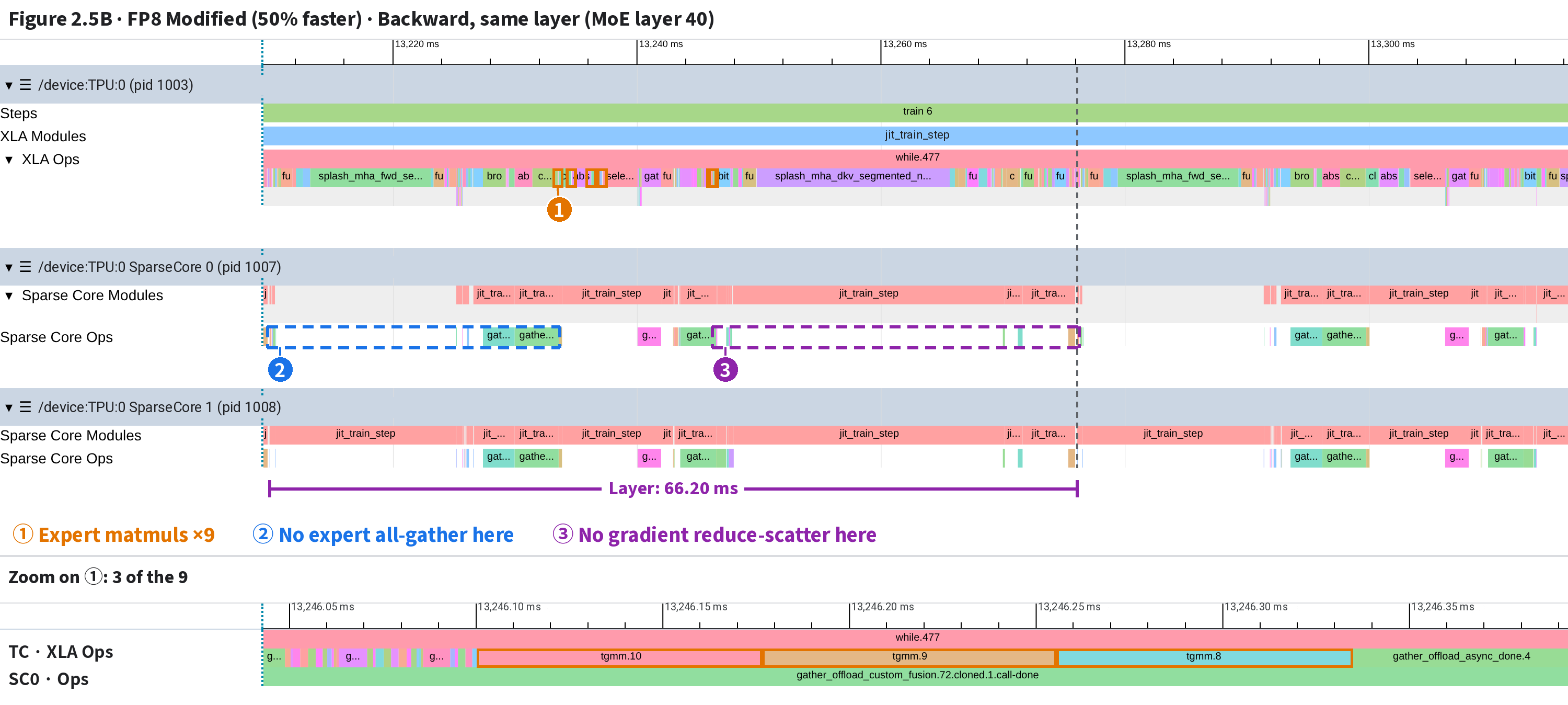
| # | What | How to tell (names and times from the xplane) |
|---|---|---|
| ① | Expert matmuls ×9 | TC: the layer’s 9 expert matmuls (gmm/tgmm) total 0.47 ms; 0.03–0.08 ms each, boxes a few pixels wide (original, same layer: 35.69 ms) Five boxes in the main image: gmm.20 (from 13,233.506 ms, 0.060 ms); gmm.22 + gmm.21 (from 13,234.596 ms, 0.037/0.037 ms); gmm.25 (from 13,236.223 ms, 0.035 ms); gmm.24 + gmm.23 (from 13,237.125 ms, 0.036/0.036 ms); tgmm.10 + tgmm.9 + tgmm.8 (from 13,246.101 ms, 0.076/0.079/0.079 ms) |
| ② | No expert all-gather here | Dashed: layer start to the first gmm, the original’s ② slot. Here SC0 has no expert-weight all-gather, only 5 other small all-gathers (none the full [1,192,…] expert set, each ≤0.16 ms) and gather_offload (gathering tokens by route) |
| ③ | No gradient reduce-scatter here | Dashed: from tgmm finishing the expert gradients to the layer end, where the original’s ③ sits. Here SC0 has not a single reduce-scatter, only 3 all-reduces (longest 0.56 ms) and 4 small all-gathers |
| Zoom 1 | Window 13,246.04–13,246.39 ms | tgmm.10 (0.076 ms), tgmm.9 (0.079 ms), tgmm.8 (0.079 ms) |
| The zoom shows only some | ① has 9 in all; the zoom boxes 3. The others are likewise tens of µs each; see row ① | |
| Bracket | Layer: 66.20 ms | Gray dashed line: end of this layer; to its right is the next layer (A and B share one window width = the original’s layer) |
reduce-scatter is the reverse: finished gradients are summed across the 64 devices in the FSDP group, and each keeps only its own share. The original’s three, in backward, have shapes like bf16[3,4096,1536]: each device keeps its 3 experts’ gradients (192 ÷ 64 = 3). The modified backward has none at all.
The screenshots box only the longest. Listing all SparseCore collectives in layer 40 in order shows if only these two kinds are missing:
📌 Windows: layer 40, forward fp8old 25,477.463–25,512.140, fp8new 9,384.636–9,410.223 ms; backward fp8old 31,199.767–31,305.887, fp8new 13,209.876–13,276.078 ms (from profile start; as in Figures 2.4 and 2.5). Counted: execution bars named with all-gather/reduce-scatter/all-reduce on the Sparse Core Ops rows of TPU:0’s two SparseCores; a same-named all-reduce on both counts once.
📌 Which op carries which weight, matched by shape against the config: [1,4096,64,128], two [1,4096,8,128], [1,64,128,4096] = attention (64 query heads, 8 KV heads, 128 per head); [1,4096,192] = router (192 experts); [1,4096,1536] ×2, [1,1536,4096] = shared expert (one, intermediate size 1,536); [1,192,4096,1536] ×2, [1,192,1536,4096] = the fully gathered expert weights. All f8e4m3fn.
📌 Reduction scope, from replica_groups in the final HLO: ⑤ reduce-scatter over {'fsdp'} (64 shards); ⑦ expert-gradient all-reduce (original all-reduce.384, modified .394, shapes bf16[3,4096,1536] ×2 + [3,1536,4096]) over {'data'} (2 replicas); the three in ⑥ (router f32[4096,192], attention, shared expert) span all 128 devices.
📌 The modified backward adds one router-weight all-gather (.499, 0.085 ms): the same weights are gathered for the recompute and again for the gradient, a compiler scheduling choice unlike the original’s [inferred]. The TensorCore’s 4 synchronous all-reduces: original all-reduce.306/307/308/312, modified .316/317/318/322 (f32[192] and a few small bf16 vectors).
| # | What is gathered or summed | Shape (f8e4m3fn gathered / bf16 gradient) | Ops per layer: Original → Modified |
|---|---|---|---|
| ① | Attention’s four weights (q, k, v, output) | [1,4096,64,128], [1,4096,8,128] ×2, [1,64,128,4096] | Fwd 4 → 4, bwd 8 → 8 |
| ② | Router weights | [1,4096,192] | Fwd 1 → 1, bwd 1 → 2 |
| ③ | Shared expert’s three weights | [1,4096,1536] ×2, [1,1536,4096] | Fwd 3 → 3, bwd 3 → 3 |
| ④ | The 192 experts’ weights | [1,192,4096,1536] ×2, [1,192,1536,4096] | Fwd 3 → 0, bwd 3 → 0 |
| ⑤ | Expert-gradient reduce-scatter | bf16[192,…] → [3,…] | Bwd 3 → 0 |
| ⑥ | Gradient sum for attention, router, shared expert (all 128 devices) | three all-reduces | Bwd 3 → 3 |
| ⑦ | Expert-gradient sum (data axis, 2 replicas) | bf16[3,4096,1536] ×2, [3,1536,4096] | Bwd 1 → 1 |
Apart from ④ and ⑤, both runs match kind for kind, and neither program has a single all-to-all: tokens never leave the device (the gather_offload moving tokens per expert is the SparseCore moving data in-device).
A new question: ⑦ is in both. The original sums first over 64 shards (⑤), then over 2 (⑦); the modified run has no ⑤, so its expert gradients are summed over only 2. Note it; Section 4 returns to the program.
⭐ Zoomed to one layer, XLA Ops level 2 is a long run of leaves: a few big labeled ones, the rest a mass of slivers. Should you click each one?
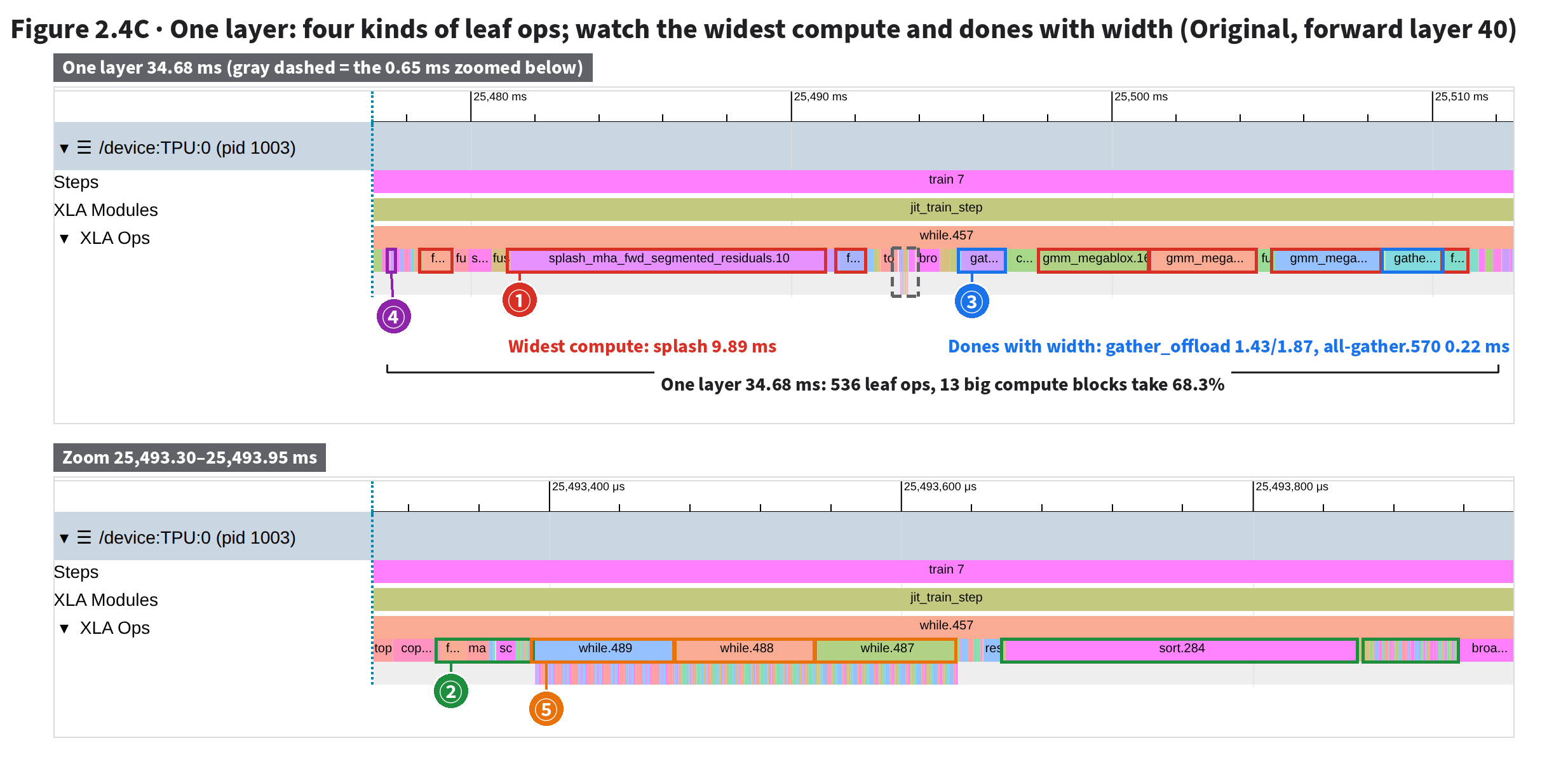
| # | What | How to tell (classified by xplane event name; counts and ms computed by r12-trace.py) |
|---|---|---|
| ① | Big compute | Pallas kernels (attention splash_mha… 9.89 ms; three expert matmuls gmm_megablox.16/17/18, 3.3–3.4 ms each) and compiler-generated matmuls, convolution fusion (9; the widest 3 boxed). This kind: 13 ops, 23.70 ms, 68.3% of the layer |
| ② | Narrow small compute (zoom window) | Elementwise, type conversion, norm, routing compares and sorts, slicing: loop fusion, reduce-window, slice, sort and the like. 315 ops, 6.79 ms, 19.6% of the layer. Layer-wide, 504 leaves are under 0.1 ms (all four kinds), totaling just 0.98 ms (2.8%). Widest in the zoom window: sort.284 (0.201 ms, the green box in the middle) |
| ③ | Data movement | gather_offload_async_done.6/.7: the TensorCore stalls here while the SparseCore moves tokens per expert (1.43/1.87 ms). Also copy-start/copy-done, relayouts like copy (data formatting; e.g. the copy.2030 block at the zoom window’s left), scatter_offload and others: 165 ops, 3.97 ms, 11.4% of the layer |
| ④ | Collectives | all-gather.570…call-done, 0.22 ms: the layer’s only collective done with width. Leaves named all-gather/reduce-scatter/all-reduce: 43 ops, 0.22 ms, 0.6% of the layer, almost all zero-width starts, dones and helper instructions around the issue |
| ⑤ | Small whiles (containers, not leaves) | while.489/488/487, about 80 µs each: loops nested in the layer, leaves one level below (Figure 2.3D counts their iterations) |
Sort this layer’s 536 leaf ops by name into the four kinds above (XLA files matmuls under convolution fusion, so they count as ①) and total each:
| Layer 40 | Layer ms | ① Big compute | ② Small compute | ③ Data movement | ④ Collectives | Of which <0.1 ms | Async dones ≥1 µs wide |
|---|---|---|---|---|---|---|---|
| Original, forward | 34.68 | 13 ops, 23.70 ms (68.3%) | 315 ops, 6.79 ms (19.6%) | 165 ops, 3.97 ms (11.4%) | 43 ops, 0.22 ms (0.6%) | 504, 0.98 ms | 4 / 27 |
| Original, backward | 106.12 | 36 ops, 72.13 ms (68.0%) | 875 ops, 24.68 ms (23.3%) | 485 ops, 7.19 ms (6.8%) | 92 ops, 2.11 ms (2.0%) | 1403, 3.42 ms | 14 / 63 |
⭐ 13 big compute ops take 68.3%; 504 slivers under 0.1 ms, just 2.8%. Only 4 of 27 async dones have width (the rest: zero width, data came early). Watch only two things: the widest compute and the dones with width.
So, three steps. Orient at the top level: click a leaf in the big loop and read tf_op: a second path segment of jvp() means forward, transpose(jvp()) backward. Find the widest compute (① above). Find the dones with width (③ ④).
To place a sliver in its module, read down a column (Figure 2.3C). The trace answers “where, and next to what”; for “a kind’s total per step”, read Op Profile / HLO Op Stats (Section 3), not slice sums on the trace.
gmm/tgmm/splash, or category convolution fusion, go to ①;
names containing a collective go to ④; copy-start/copy-done, category data formatting, names containing gather_offload/scatter_offload/sparse-core-data-format, and dynamic-slice/dynamic-update-slice starts and dones go to ③ (plain copy ops of category data formatting too); the rest go to ②.
Custom-calls named prepare_… follow the communication or transfer in their name; all under 1 µs wide.copy-done (each under 1.1 µs); of the async dones with width, only 1 is a collective.
Backward, 14 of 63 async dones exceed 1 µs; the widest are a dynamic-slice-done at 4.68 ms and the all-gather.548…call-done from 2.5 at 1.18 ms.| Layer 40 | Layer ms | ① Big compute | ② Small compute | ③ Data movement | ④ Collectives | Of which <0.1 ms | Async dones ≥1 µs wide |
|---|---|---|---|---|---|---|---|
| Modified, forward | 25.59 | 13 ops, 13.68 ms (53.5%) | 262 ops, 7.80 ms (30.5%) | 90 ops, 3.92 ms (15.3%) | 32 ops, 0.18 ms (0.7%) | 369, 1.14 ms | 4 / 23 |
| Modified, backward | 66.20 | 36 ops, 37.27 ms (56.3%) | 872 ops, 25.56 ms (38.6%) | 485 ops, 2.71 ms (4.1%) | 72 ops, 0.66 ms (1.0%) | 1392, 3.85 ms | 12 / 57 |
Modified: ① is still 13/36 ops (names still start with gmm), but each expert matmul is down to tens of µs; ①’s share falls from 68.3% to 53.5% forward, 68.0% to 56.3% backward. The kind table shows the same work got thinner, not why; for why, see 2.4 and Section 3.
fp8old, view_start=25,476.963, view_end=25,512.640 (as in 2.4).fp8old, view_start=25,493.300, view_end=25,493.950; click sort.284 and gather_offload_async_done.6 (one-layer screen); read Wall Duration.⭐ The modified layer’s SparseCore lacks two kinds of communication; expert matmuls shrink to 1/75–1/93: a big chunk of work is gone. Is all the missing 3.9 s this undone work? Section 3 checks the totals.
fp8old view_start=25476.963, view_end=25512.640 ↗ Open; fp8new 9384.136–9419.813 ↗ Open. Modified, zoom windows: 9404.183–9404.423 ↗ Open, 9405.183–9405.423 ↗ Open.fp8old 31199.267–31306.387 ↗ Open; fp8new 13209.376–13316.496 ↗ Open; modified zoom window 13246.043–13246.393 ↗ Open.gmm_megablox.16 (TensorCore) and all-gather.575 (SparseCore); read Wall Duration (ns) in Details.⭐ Per step the original’s TensorCore waits on communication dones only 161 ms (1.4%): compute hides most transfers. The modified recipe saves just 119 ms of that wait, far short of 3.9 s.
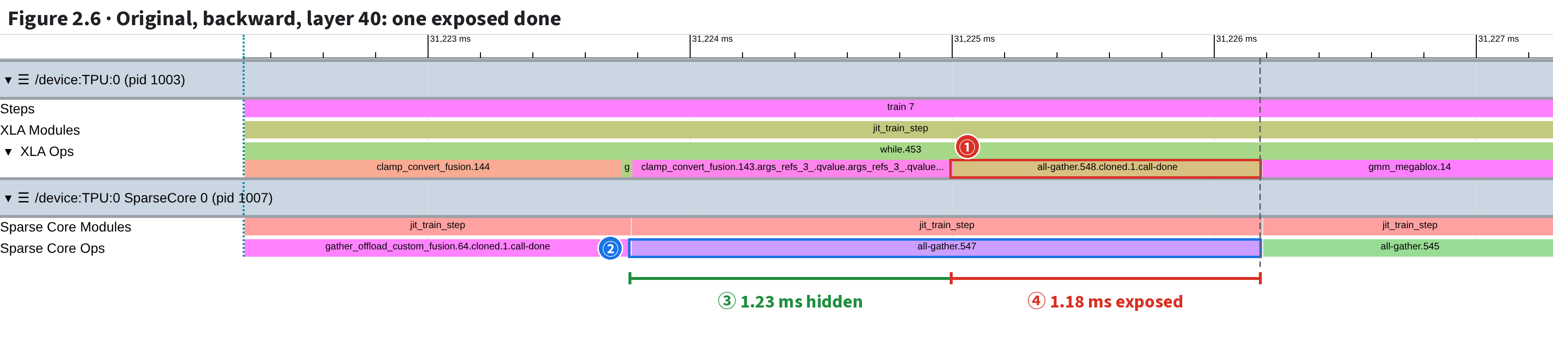
| # | What | How to tell (names and times from the xplane) |
|---|---|---|
| ① | Done on the TC | TC: all-gather.548.cloned.1.call-done, 31,225.002–31,226.183 ms, 1.181 ms |
| ② | Execution bar on SC0 | SC0: all-gather.547 (one below the TC’s number), 31,223.777–31,226.183 ms, 2.406 ms, shape f8e4m3fn[1,192,4096,1536]: a gather of all 192 experts’ weights |
| ③ | Hidden part | SC starts moving → TC reaches done: 1.225 ms, overlapped with TC compute |
| ④ | Exposed part | Done width 1.181 ms: the TC stalls until the SC finishes. Dashed line: right edges 0.1 µs apart |
The static figure shows only the outcome. Replayed from start: the SparseCore row is still busy, so 547 starts moving over 4 ms late; the TensorCore keeps computing, reaches done before the transfer ends, and waits.
| Stop | What happens | Reading |
|---|---|---|
| 1 | 0 ms: TensorCore issues start, keeps computing | Start has almost no width |
| 2 | SparseCore row still moving tokens per expert (two gather_offload); 547 starts only at 4.27 ms | Starts only at 4.27 ms (why the two ahead block it: [inferred: the SparseCore row runs one at a time]) |
| 3 | SparseCore moves 547; TensorCore quantizes | 1.23 ms hidden |
| 4 | TensorCore reaches done; 547 unfinished | 1.18 ms exposed: done and 547 right edges 0.1 µs apart |
| 5 | Released, runs gmm_megablox.14 | Its operand 7 is the done of all-gather.548 (HLO) |
| 6 | Per-step total | TensorCore wait on communication dones 161.0 → 41.6 ms: 119 ms saved, far short of 3.9 s |
all-gather.547 ↔ all-gather.548…call-done), and their right edges align: the TensorCore’s wait ends as the SparseCore finishes. Here the gap is 0.1 µs.gather_offload ops; 547 starts 3 µs after the previous one ends: it looks like a queue [inferred: the SparseCore row runs one at a time]. Start is at 31,219.51 ms, left of the Figure 2.6 window (the animation’s time zero).fp8old, view_start=31222.3, view_end=31227.3 ↗ Open; click all-gather.548.cloned.1.call-done and press m to mark its span on the ruler: its right edge lines up with all-gather.547 on the SparseCore.In one layer, Section 2 saw the SparseCore’s expert gather and gradient scatter vanish and expert matmuls shrink to 1/75–1/93. But a layer is one of 78 iterations. Is the step’s missing 3.9 s all undone work? Check on two pages that report totals: Op Profile by category, Op Stats by op.
⭐ One minute: Op Profile by category, both runs → expand custom-call → click for details → Op Stats: rank, count.
| Stop | Page, action | Reading |
|---|---|---|
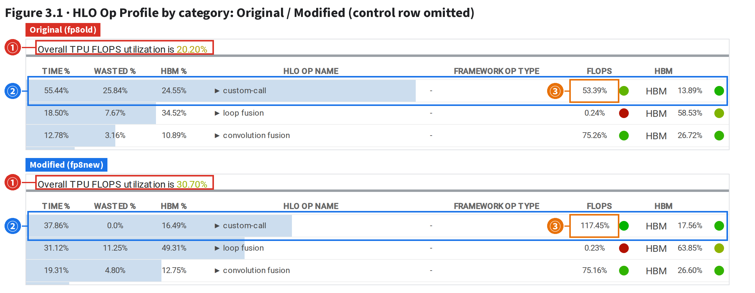
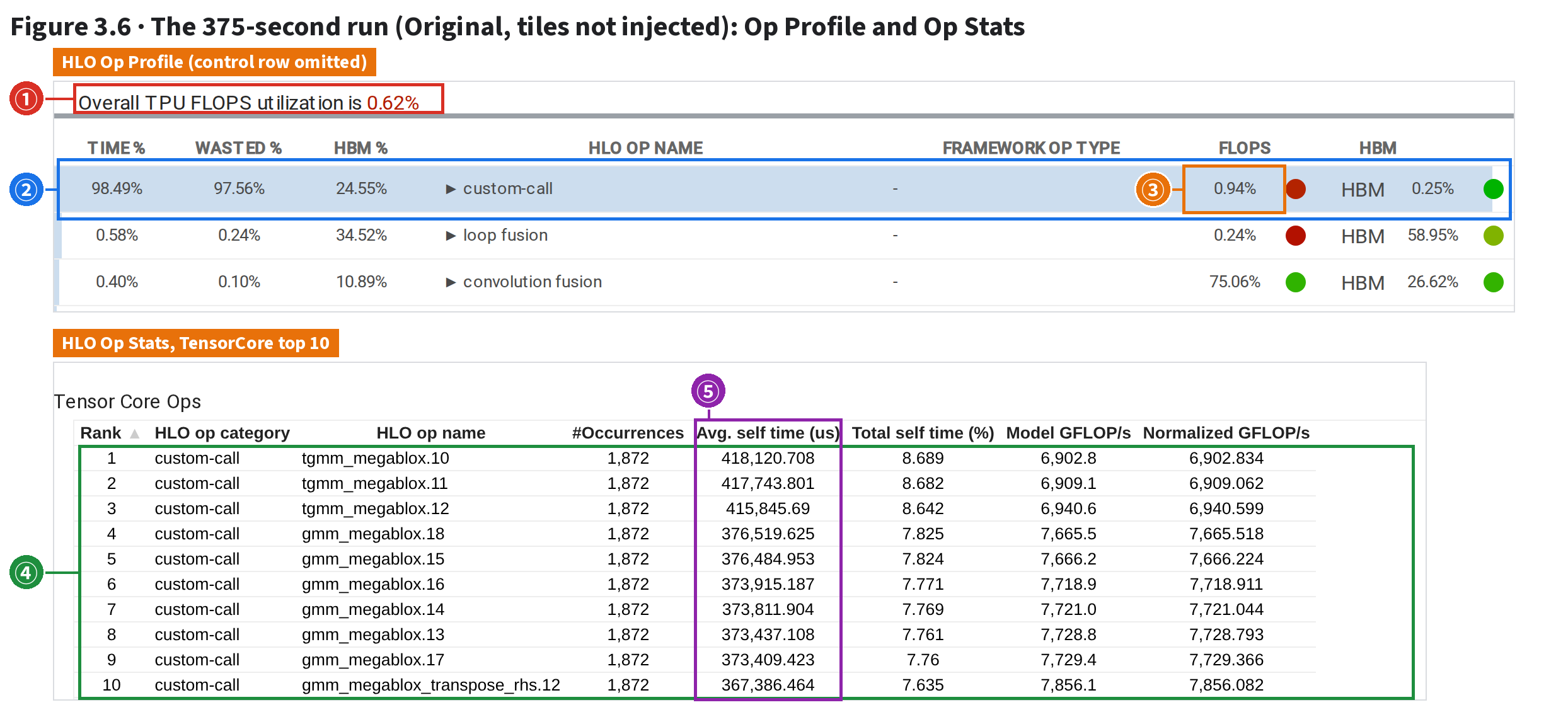
| 1 | Original, HLO Op Profile, Group by: Category | Overall FLOPS utilization 20.20%; custom-call 55.44% of time, 53.39% utilization |
| 2 | Modified, same page | custom-call 37.86% of time, utilization 117.45%, WASTED 0.0% |
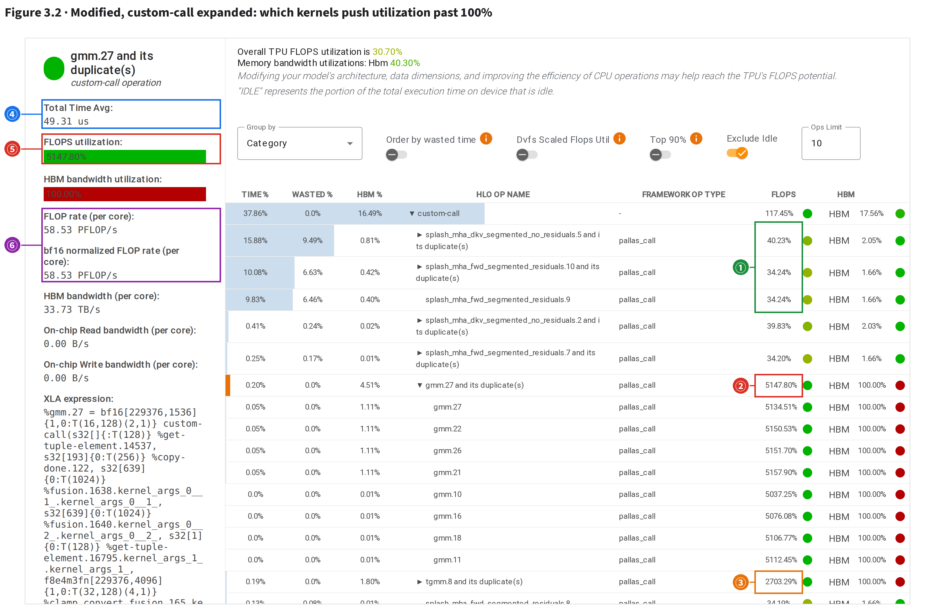
| 3 | Click custom-call to expand | Attention, three groups: 34–40%, as in the original; gmm.27 group 5,147.80%, tgmm.8 group 2,703.29% |
| 4 | Click the gmm.27 row; read the left panel | 49.31 µs per call, 58.53 PFLOP/s: 25× FP8 peak |
| 5 | Original, expanded the same way | Same expert matmuls: 2.4–8.8% of time per group, 45–77% utilization |
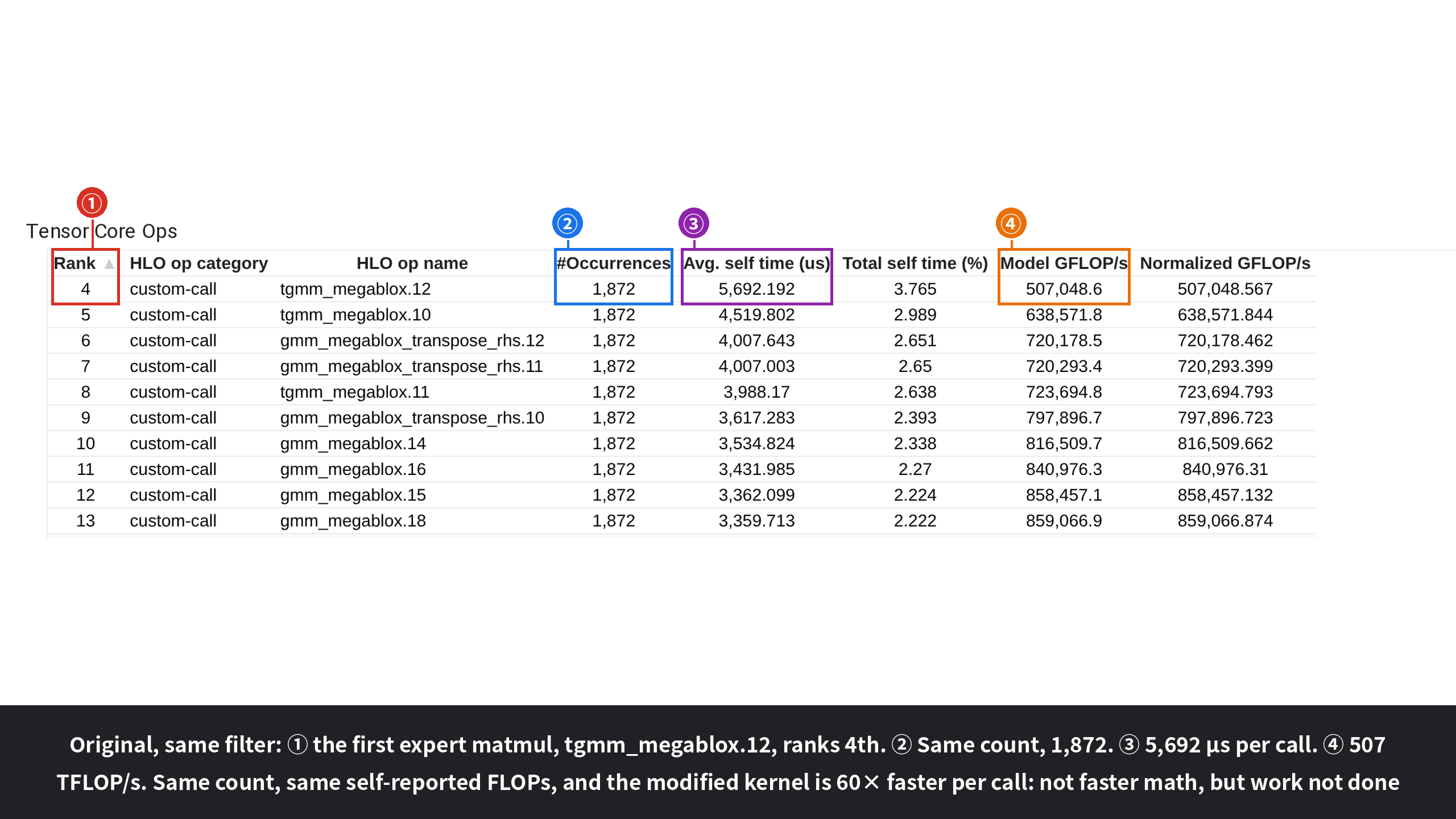
| 6 | Modified, HLO Op Stats, name filter gmm | First expert matmul ranks 124th; 1,872 calls; 94.5 µs per call |
| 7 | Original, same filter | Ranks 4th; the same 1,872 calls; 5,692 µs per call |
Full video: topic07-xrec-opprof.en.mp4 (last frame png). Below, stop by stop.
⭐ Nearly all the missing time is in custom-call: 6.5 s → 3.0 s per step. Yet its utilization rises instead, to 117.45%.

| # | What | On the page (boxes at the on-page text) |
|---|---|---|
| ① | Overall FLOPS utilization | Overall TPU FLOPS utilization: original 20.20%, modified 30.70% |
| ② | The custom-call category | Pallas kernels: TIME 55.44% → 37.86% (in ms, Op Stats basis, mean of 8 TensorCores × 3 steps: 6532.9 → 2969.9 ms per step); WASTED 25.84% → 0.0% (wasted = time share × (1 − max(FLOPS utilization, HBM utilization)); above 100% utilization it is scored as no waste at all) |
| ③ | custom-call FLOPS | Category FLOPS utilization 53.39% → 117.45%, above the page’s own peak |
HLO Op Profile buckets every TensorCore instruction by category, with two numbers each: TIME % (share of TensorCore time) and FLOPS (utilization; formula below). custom-call is an external kernel XLA calls rather than generates: here, hand-written Pallas kernels, both attention (splash) and the expert matmuls (gmm: forward and input gradient; tgmm: expert-weight gradient; glossary in 0.3). custom-call alone loses 3.6 s per step (6,532.9 → 2,969.9 ms, table ②); the rest together barely move.
The odd part is the third column: time fell by over half, yet utilization rose from 53.39% to 117.45%. Utilization above 100% means more operations per second than the page’s own peak. Don’t conclude yet; expand it.
pl.CostEstimate, stored in the compiled HLO as cost_estimate).fp8old/fp8new, tool op_profile: http://127.0.0.1:6311/?run=fp8old/2026_08_15_03_57_28&tag=op_profile&host=gke-node-1 (for the modified run, change the run and timestamp to fp8new/2026_08_15_04_11_46); ☰ at top left collapses the sidebar.⭐ Two expert-matmul kernels drag the utilization up. The gmm.27 group takes 49.31 µs per call, i.e. 58.53 PFLOP/s: 25× the FP8 peak. No chip can do that; the kernel did not do all the work it reports.

| # | What | On the page (boxes at the on-page text) |
|---|---|---|
| ① | Three attention kernels | Three splash_mha_dkv/fwd groups: FLOPS 40.23%, 34.24%, 34.24%, as in the original (Op Stats per call: 15,788/9,886 µs original, 15,773/9,885 µs modified) |
| ② | The gmm.27 group | gmm.27 and its duplicate(s): TIME 0.20%, FLOPS 5,147.80% (expanded: gmm.27/22/26/21, 5,134–5,158% each) |
| ③ | The tgmm.8 group | tgmm.8 and its duplicate(s): FLOPS 2,703.29% |
| ④ | Total Time Avg | Left panel: this group averages 49.31 µs per call |
| ⑤ | FLOPS utilization | Left panel: 5,147.80%. HBM bandwidth utilization is also 100.00% (next line: 33.73 TB/s vs a per-core peak of 3,433 GiB/s ≈ 3.69 TB/s, also impossible) |
| ⑥ | FLOP rate | Left panel: 58.53 PFLOP/s = self-reported 2.886 TFLOP per call ÷ 49.31 µs. The bf16 normalized rate is also 58.53: Pallas kernels aren't rescaled by precision |
Expanded, custom-call's time goes mostly to three attention kernels at 34–40% utilization, nearly as in the original recipe. The absurd rows are two expert matmuls with only 0.2% of the time (②③). The 117% is an average: a big honest attention block (about 37%) plus a small absurd expert-matmul block (about 2,500%) lands above 100%.
Why it is impossible. The numerator is self-reported: the compiled program records 2,886,218,022,912 FLOPs per gmm.27 call = 2 × 229,376 × 4,096 × 1,536.
The 229,376 rows are this device's tokens (7 × 4,096), each routed to 8 experts; 4,096 and 1,536 are an expert matrix's two dimensions. The count comes purely from input shapes, however many experts were actually computed.
The denominator is measured: 49.31 µs per call, so 58.53 PFLOP/s. TPU v7's official FP8 peak is 4,614 TFLOP/s per chip, 2,307 TFLOP/s per core (2 TensorCores per chip): 25× over.
HBM likewise: 33.73 TB/s against about 3.69 TB/s per core (⑤), 9× over.
Same kernel, another page: the Roofline Model page plots each op as a point on §1's roofline. A kernel doing real work at best touches the roof; gmm.27 lands off the chart (recording stop 3).
| Stop | Action | What you see |
|---|---|---|
| 1 | Modified, Roofline page, Device Information at the top | Peak 1,028.75 TFLOP/s per core; Time Scale Multiplier 1.10529 (Op Profile's peak ≈ the product) |
| 2 | Original, down to Section2, type gmm_megablox.16 in the Operation box | One blue dot on the flat roof; 840,976 GFLOP/s, 81.7% of peak |
| 3 | Modified, same box, type gmm.27 | No dot: 58,380,995 GFLOP/s is 57× above the flat roof, off the chart; the table shows 5,674.9%, memory bandwidth 912.6% |
| 4 | Just that table row | 58,380,995 ÷ 1,028,750 = 56.7×; code at MaxText backend.py (modified branch) |
⭐ Same FLOPs booked, less work done: both FP8 runs book identical custom-call FLOPs, yet its time fell from 6,541.8 ms to 2,972.8 ms. Utilization = same numerator ÷ shrunken denominator, hence the 117%.
| Per step, per TensorCore | Original | Modified | Source |
|---|---|---|---|
| custom-call booked FLOPs (TFLOP) | 3,966.1 | 3,966.1 | 18 cost_estimate (hlo_proto) × TPU:0 calls/step |
| of which expert matmul / attention | 2,762.1/1,204.0 | 2,762.1/1,204.0 | |
| custom-call measured time (ms) | 6,541.8 | 2,972.8 | TPU:0, mean of 3 steps |
| Utilization on the page | 53.39% | 117.45% | Op Profile |
| One expert matmul: time per call | 3,431.1 µs (gmm_megablox.16) | 48.6 µs (gmm.27) | Same |
| self-reported 2.886 TFLOP ÷ that time | 841 TFLOP/s | 59,387 TFLOP/s | Arithmetic |
The table's per-call time for one expert matmul is a 3-step mean on TPU:0 (gmm.27: 48.6 µs); the left panel's 49.31 µs averages the group over 8 cores: 1–2% apart.
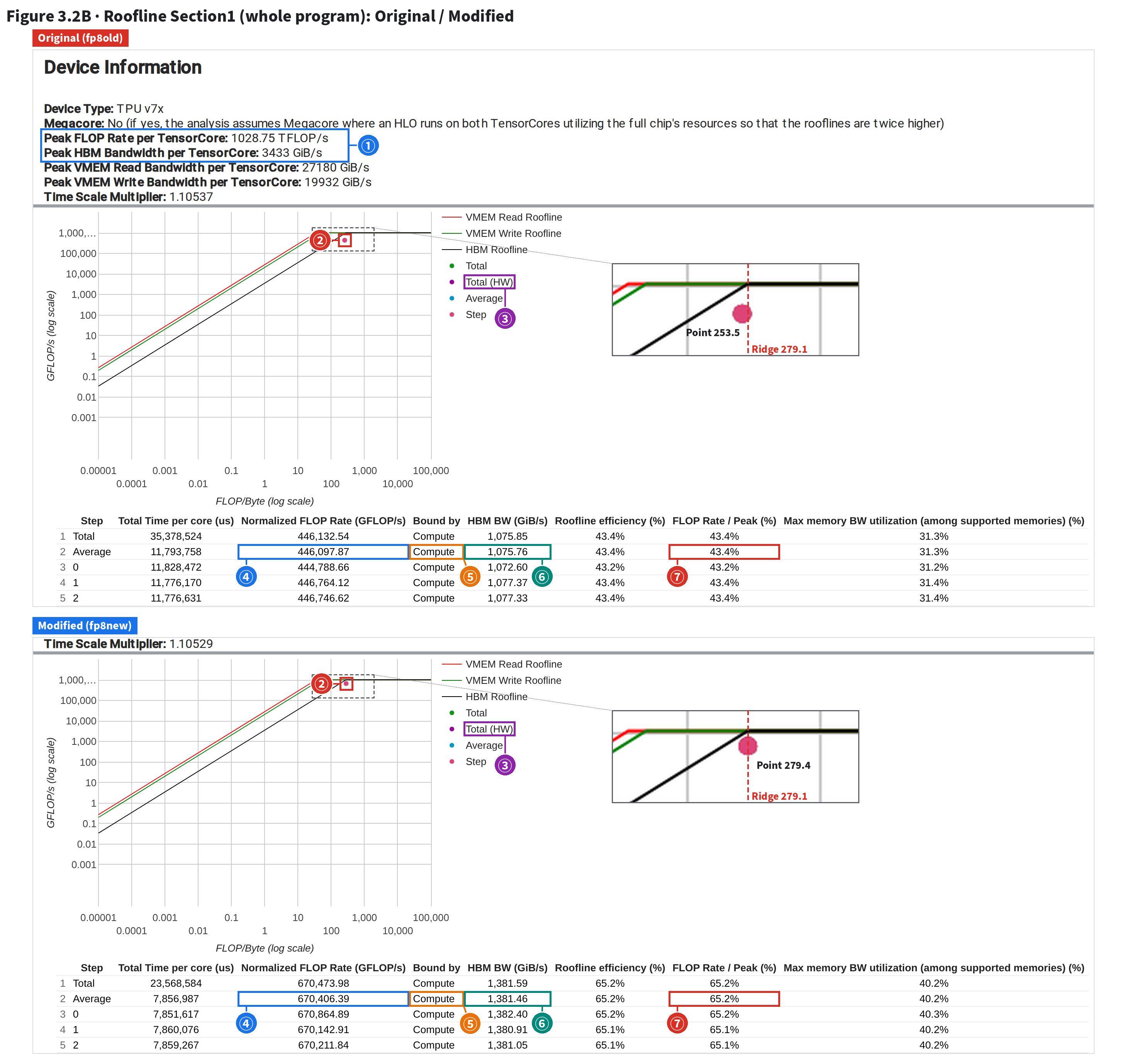
custom-call row to expand it, then gmm.27 and its duplicate(s): the left panel shows ④⑤⑥.roofline_model, in Section2 type gmm.27 in the Operation box (original: gmm_megablox.16), press Enter.⭐ The step average is inflated too: Roofline Section1 shows 43.4% → 65.2%. Same cause as the 117%: both runs book nearly equal FLOPs per step (5,261 vs 5,267 TFLOP) in a step 66.6% as long. Without expert matmuls the rest goes 29.9% → 31.4%, barely moving.
Recall §1's roofline: arithmetic intensity (operations per byte moved) on x, operations per second on y. The left slope is the bandwidth limit, the flat right part the compute limit; they meet at its ridge point. XProf's Roofline page draws it over a profile: Section1 plots the whole program as one point, Section2 each of the 1000 most expensive ops. The y numerator is booked FLOPs (same source as Op Profile), the denominator measured time. That is why gmm.27 (§3.2) can land off the chart, and the step average cannot escape the same problem. Section1 first, the two runs stacked:

| # | What | On the page (boxes at the on-page text; points read off the axes) |
|---|---|---|
| ① | Peak (denominator) | Per TensorCore 1,028.75 TFLOP/s, HBM 3,433 GiB/s; their ratio is the ridge point, 279.1 FLOP/Byte (page's HBM Roofline ridge point: 279.085). Time Scale Multiplier 1.10537 original, 1.10529 modified (see below) |
| ② | Where the step lands | Three points overlap (Total, Average, each Step): x = 253.5 → 279.4 FLOP/Byte, right by the 279.1 ridge point; y = 446,098 → 670,406 GFLOP/s, a clear step up |
| ③ | Total (HW) | In the legend, yet no point and no table row: it needs whole-session hardware-counter FLOPs (page note (5)), which open-source XProf 2.23.1 gives for neither run. Only the Total/Average rows are usable |
| ④ | Normalized FLOP Rate | Average row (complete steps only): 446,097.87 → 670,406.39 GFLOP/s. Times the step time (11.794 s / 7.857 s): 5,261 / 5,267 TFLOP booked per step per core, almost identical |
| ⑤ | Bound by | Both Compute: XProf picks the higher utilization (compute 43.4%/65.2% vs HBM 31.3%/40.2%) |
| ⑥ | HBM BW | 1,075.76 → 1,381.46 GiB/s; ÷ 3,433 = 31.3% → 40.2%, the rightmost column, Max memory BW utilization |
| ⑦ | FLOP Rate / Peak | 43.4% → 65.2%: 446,098 ÷ 1,028,750 = 43.36%, 670,406 ÷ 1,028,750 = 65.17%. Numerator (FLOPs booked per step) unchanged, denominator (step time) down to 66.6%, so the ratio rose 1.50× |
Read the Average row (complete steps only; Total includes partially captured ones). Normalized FLOP Rate is booked FLOPs per second; Bound by, whether compute or bandwidth is closer to its limit; FLOP Rate / Peak, the rate ÷ the 1,028.75 TFLOP/s per-core peak. Both runs say Compute and utilization jumps, as if the whole step really got much faster.
Work out the numerator first (FLOPs per second × step time): 5,261 vs 5,267 TFLOP per step per core, 0.1% apart. Same work, a third less time: utilization up 1.50×. Same accounting as §3.2's 117%: each expert matmul is booked at 2.886 TFLOP from its shapes; the modified calls shrink to tens of µs, the booking doesn't. Remove the expert-matmul family from numerator and denominator and the rest runs at 29.9% of peak original, 31.4% modified: the 21.8-point step gain is almost all this one family.
| Per step, per TensorCore | Original | Modified | How derived |
|---|---|---|---|
| Booked FLOPs (TFLOP) | 5,261 | 5,267 | Average row Normalized FLOP Rate × step time |
| Step time (ms) | 11,794 | 7,857 | Average row Total Time per core |
| FLOP Rate / Peak | 43.36% | 65.17% | ÷ 1,028,750 GFLOP/s; page: 43.4%/65.2% |
| of which expert matmul: FLOPs / time | 2,762.1/3,665.7 ms | 2,762.1/98.3 ms | xplane, 3 complete TensorCore steps (table in §3.2) |
| everything except expert matmul | 29.9% | 31.4% | (total FLOPs − family) ÷ (total time − family) ÷ peak our derivation |
bytes_accessed (table's Memory BW, 1,638.91 GiB/s); Bound by uses the HBM bytes of a second, per-memory-space count (table's HBM BW, 1,075.76 GiB/s). By that count intensity is 386.2, right of the ridge, and compute utilization (43.4%) beats HBM (31.3%), hence Compute. The two byte counts differ, for single kernels in Section2 too.SetRooflineMetrics in open-source XProf's xprof/convert/op_metrics_to_record.h (openxla/xprof, tag xprof-v2.23.1), summarized:
operational_intensity = flops_v2 / bytes_accessed # x-axis: self-reported bytes
hbm_bytes = sum of each instruction's HBM entries in memory_accessed_breakdown # else falls back to bytes_accessed
hbm_bw = hbm_bytes / time # the table's HBM BW
flops_utilization = measured_flop_rate / peak_flops
hbm_bw_utilization = hbm_bw / peak_hbm_bw
Bound by = the highest utilization (Compute, HBM; on TPU also CMEM and VMEM when they have bytes)
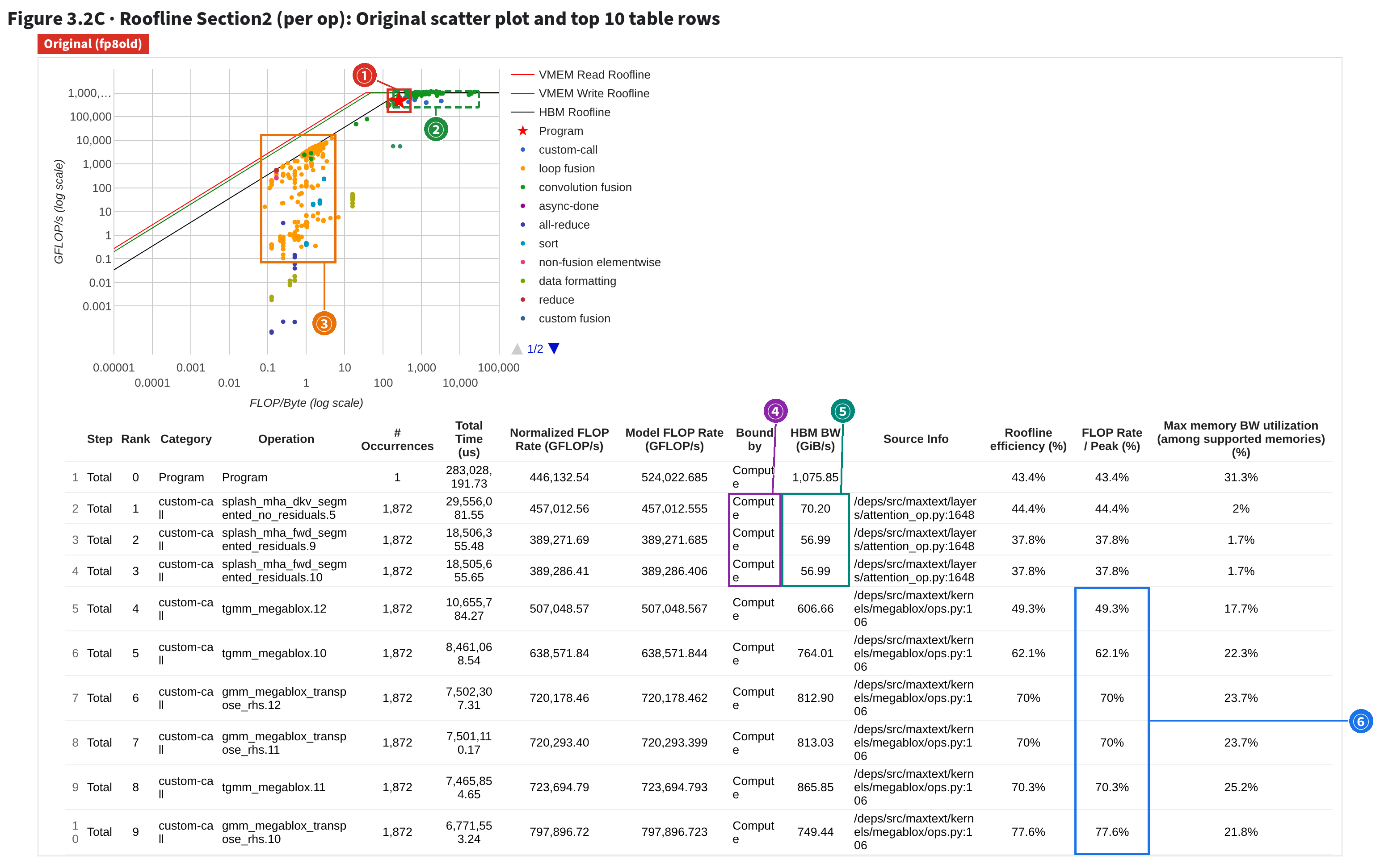
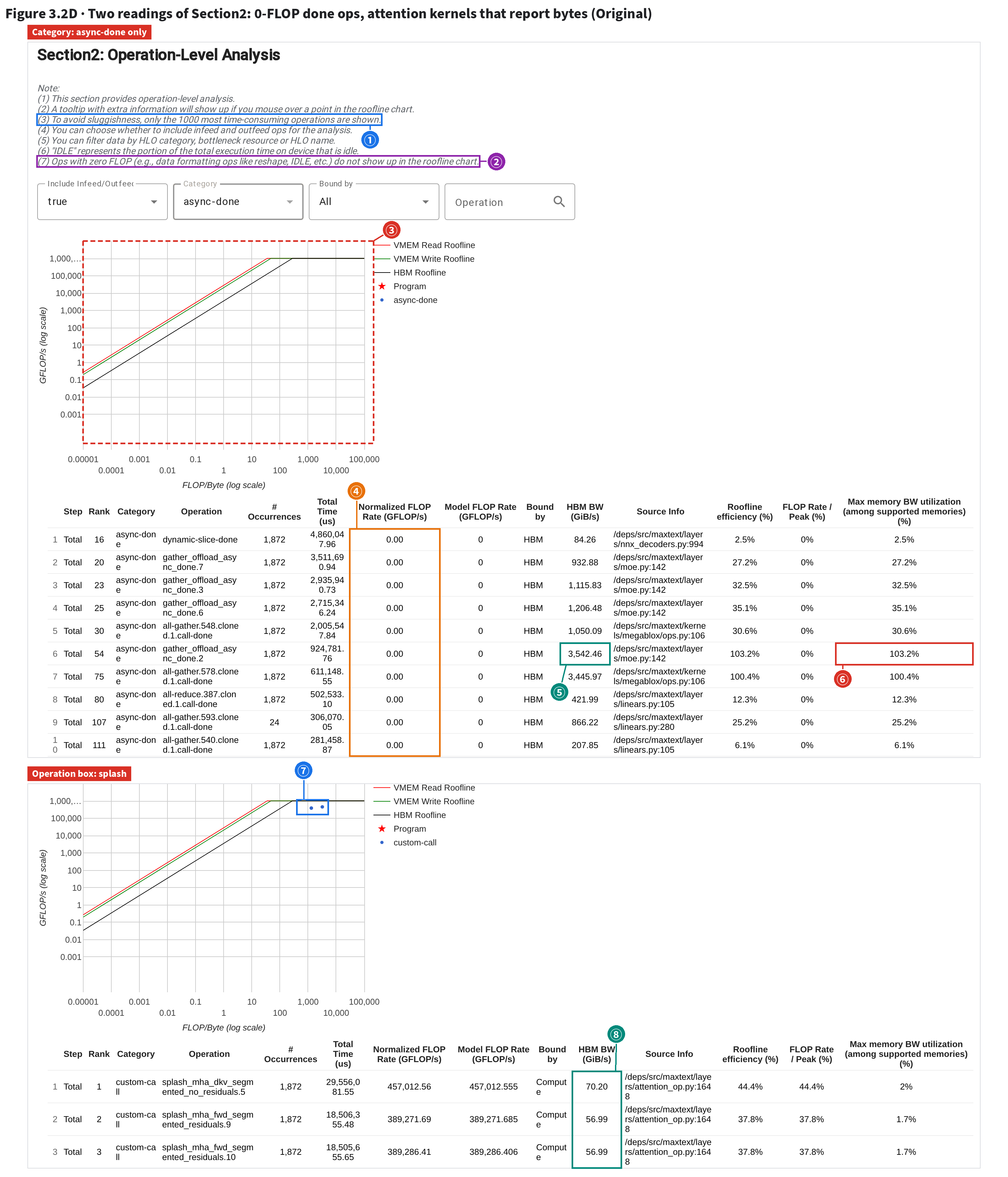
So Bound by only says which term is closer to its limit; both numerators are booked, not a measured bottleneck. Division by zero yields 0 (SafeDivide).fp8old, tool roofline_model: http://127.0.0.1:6311/?run=fp8old/2026_08_15_03_57_28&tag=roofline_model&host=gke-node-1. Collapse the sidebar with ☰ (top left) to see Device Information and Section1 at the top.fp8new/2026_08_15_04_11_46. Hover over a point to see its row's numbers.⭐ Per op, the original's points all behave: matmuls hug the flat roof, elementwise fusions the slope. Two kinds of “fake points” sit far from the roof: 0-FLOP done ops (they can't be plotted at all) and done rows over 100% bandwidth. Attention kernels report bytes, so their Bound by is trustworthy.
Scroll down to Section2. One point per op, colored by category; the table is sorted by total time, 10 rows a page. On the original, read the chart's shape first, then the top rows:

| # | What | What the page shows (boxes at the on-page text; points read off the axes) |
|---|---|---|
| ① | Red star: whole program | The same point as in Section1 (intensity 253.5, 446,133 GFLOP/s) |
| ② | A string along the flat roof | Blue custom-call points (44, intensity 240–3,210) and green convolution fusions (XLA's own matmuls; 112 of 134 marked Compute) crowd right of the ridge point, along the flat roof. Time-weighted, custom-call averages 59.0% of peak, convolution fusion 83.2%. Matmuls doing real work belong exactly here |
| ③ | A cloud along the slope | Orange loop fusions (elementwise fusions, 435): intensity only 0.08–4.6, 425 marked HBM, time-weighted at 61.3% of HBM peak. Little compute, lots of movement: the only lever is fewer reads and writes |
| ④ | Top three: attention kernels | splash_mha_dkv/fwd (Pallas kernels): Bound by Compute, FLOP Rate/Peak 44.4%/37.8% |
| ⑤ | Their HBM BW | 70.20/56.99 GiB/s, not 0: splash reports bytes in cost_estimate (details below), so Bound by for these can be trusted |
| ⑥ | Ranks 4–9: expert matmuls | tgmm/gmm_megablox (Pallas): FLOP Rate/Peak 49.3%–77.6%, all below 100%. Modified, the same family's gmm.27 is at 5,674.9% (§3.2 recording stop 3) |
A convolution fusion is a matmul XLA fused with its neighboring small ops; a loop fusion, a chain of elementwise ops fused into one; a custom-call, a Pallas kernel. The matmul string sits right of the ridge: much compute, little movement, so at best it nears the flat roof (custom-call 59.0%, convolution fusion 83.2%, ②). The elementwise cloud has intensity below 5: each value loaded gets only a few operations, so only fewer reads and writes help. On the original, this chart rules things out: ordinary ops already sit on the roof; no category “clearly could go faster”.
Two more readings. First, done ops (§2: where the TensorCore waits for an async job, mostly a SparseCore transfer): select only async-done under Category, and the chart is empty. Second, the attention kernels: type splash in the Operation box.

| # | What | What the page shows (boxes at the on-page text; points read off the axes) |
|---|---|---|
| ① | Only the top 1000 plotted | Page note (3): Section2 takes only the 1000 most time-consuming ops. Of the original's 3,897 TensorCore ops the table has 999 rows, dropping only 0.21% of self time (74 ms per core of the whole profile's 35,379 ms), so category shares hold: custom-call 55.5% here vs 55.4% in the full Op Stats. Open-source 2.23.1 has no pie chart on this page |
| ② | 0 FLOPs not plotted | Page note (7): ops with 0 FLOPs get no point. The top 1000 rows include 263 of them (loop fusion 78, data formatting 35, slice 34, async-done 32…), 10.3% of total time |
| ③ | Empty chart | With only async-done selected, the chart below shows no points at all: every done has 0 FLOPs |
| ④ | FLOPs 0, Bound by HBM | All 32 done rows show 0.00 GFLOP/s and Bound by HBM, the only nonzero term. A done is where the TensorCore waits for an async job to finish (mostly a SparseCore transfer). Skip it; see in Trace Viewer what it waited on |
| ⑤ | The done's HBM BW | gather_offload_async_done.2: 3,542.46 GiB/s, above the 3,433 peak |
| ⑥ | Over 100% | 103.2%: the numerator is the 1,879,048,192 bytes booked to this done from its shapes, the denominator only the TensorCore's short wait on it (494.0 µs per call): two different things |
| ⑦ | Points of the two attention kernels | dkv (intensity 3,210) and fwd (1,304) both plot as blue points: the kernels report bytes, so intensity = FLOPs ÷ bytes has a value |
| ⑧ | HBM BW not 0 | 70.20/56.99 GiB/s. For a Pallas kernel, check whether this cell is 0 before reading Bound by. Here it isn't, so Compute is credible |
Three rules (details in the two tables above). Skip done ops: FLOPs are 0 and the bandwidth cell is meaningless too (gather_offload_async_done.2: shape-booked bytes ÷ the TensorCore's 494 µs wait, ⑤⑥); see what it waits on in Trace Viewer (§2.5).
For a Pallas kernel, first check whether HBM BW is 0. If the author left bytes out of pl.CostEstimate, Bound by has only compute to go on and Compute means nothing. Ours all fill them in (none of either run's 18 cost_estimate entries has 0 bytes), so splash's 44.4%/37.8% reads at face value.
Is the top 1000 enough? The table holds only 999 of the original's 3,897 TensorCore ops, yet drops just 0.21% of time (0.31% modified); custom-call's share is 55.5% vs 55.4% in full Op Stats. A profile with many small ops may not be covered as well; for shares, Op Stats is safer.
bytes_accessed ÷ time per call; HBM BW = the HBM part of the per-memory-space byte count each instruction carries in the xplane (memory_access_breakdown) ÷ time per call. Recomputed, both match the page digit for digit:
splash_mha_dkv…5 self-reports 2,247,884,800 bytes → 132.60 GiB/s, HBM count 1,190,133,764 → 70.20 GiB/s; gmm_megablox.16 self-reports 5,664,411,648 → 1,537.13 GiB/s, HBM count (two entries combined) 2,852,140,804 → 773.97 GiB/s. The point's x uses the first (dkv: 3,209.9 FLOP/Byte), Bound by the second.cost_estimate entries keep the original's flops exactly, but several expert-matmul entries report fewer bytes (smallest 1,681,922,048 vs 4,060,184,576 original). Once the input shape becomes [3,…], the shape-derived byte count follows; the FLOP formula doesn't [inferred: from comparing the two sets of values; we did not read how the kernel source computes either].async-done in the Category drop-down. Bottom: set Category back to All, type splash in the Operation box and press Enter. Ignore the table's Program ID column (hidden in the screenshots).Utilization Viewer (per the official docs, it charts how busy each execution unit is) shows No Data for every profile in open-source 2.23.1: this version routes it to an unregistered processor (log: No ProfileProcessor registered for tool: utilization_viewer), fixed in 2.23.2. The raw data is in these 7 profiles (hardware-counter events on the TPU plane), but our screenshots use 2.23.1, so we skip the page. Its question, does the MXU really run FP8, we answer from the kernel's HLO operand types (f8e4m3fn[3,4096,1536] in Details) and the single kernel's FLOP rate (§3.2).
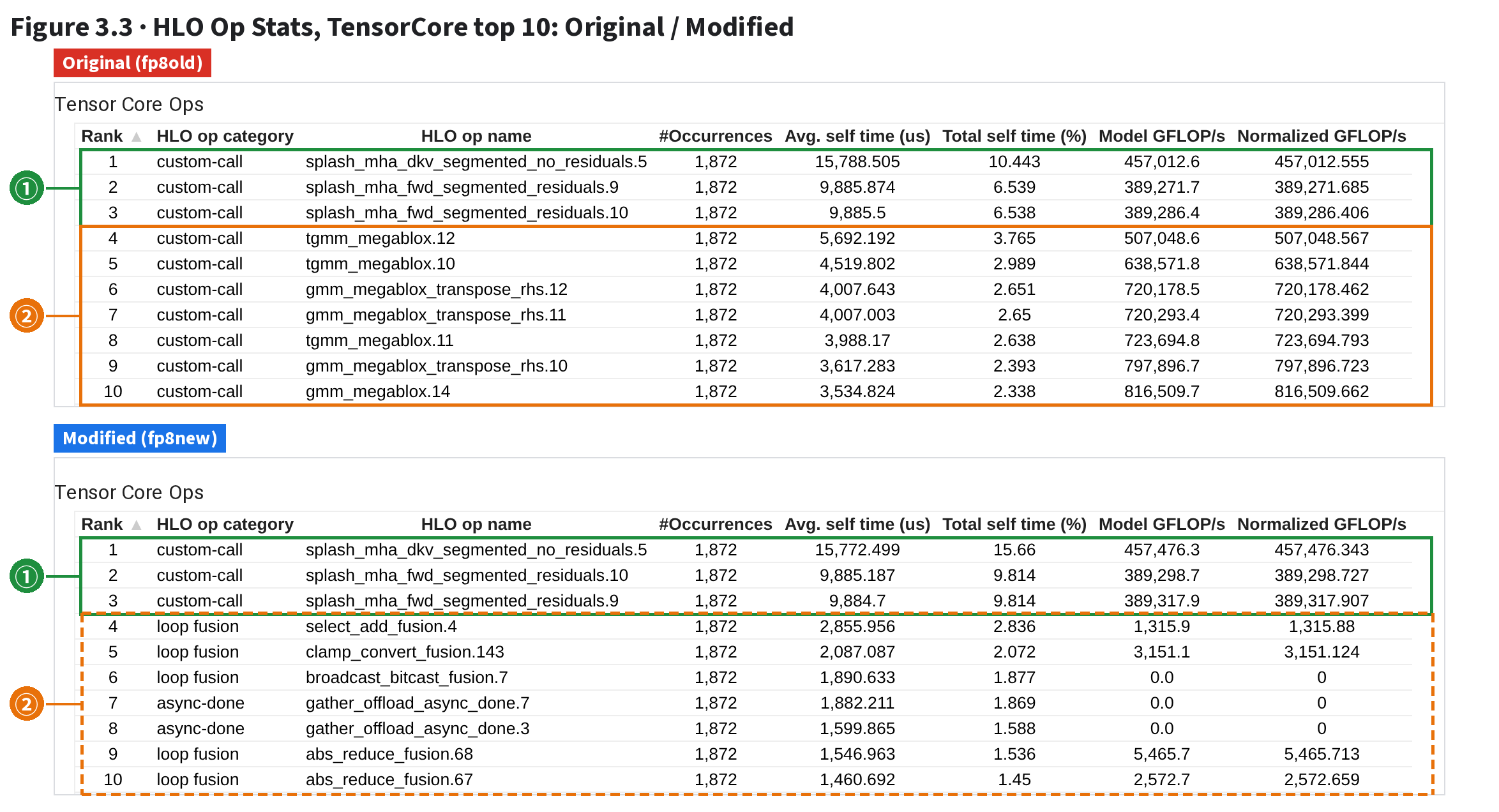
⭐ Expert matmul calls didn't drop (1,872 in both), but each fell from a few ms to tens of µs, 100 at most. The SparseCore's expert-gradient reduce-scatters are gone.

| # | What | On the page (boxes at the on-page text) |
|---|---|---|
| ① | Top three: attention | Both runs: splash attention kernels, 15,788/9,886/9,886 vs 15,773/9,885/9,885 µs per call. Same work, same time (the control) |
| ② | Ranks 4–10: expert matmuls | 7 of the original's top 10 are expert matmuls (tgmm_megablox/gmm_megablox_transpose_rhs/gmm_megablox), 3.5–5.7 ms per call. Modified: none in the top 10; ranks 4–10 are loop fusions and gather_offload async-dones, and the first expert matmul, tgmm.8, is 124th (Figure 3.4). The modified ② is dashed: no expert matmuls left at those ranks |
HLO Op Stats is one big table, a row per op: call count (#Occurrences), self time per call (excluding nested sub-instructions), share and FLOP rate.
The modified top 10 has no expert matmuls (②); ranks 4–10 go to loop fusions (a chain of elementwise ops fused into one) and gather_offload, which moves tokens to their experts.
The top three, the attention kernels, barely differ; as the control, they show nothing else moved.
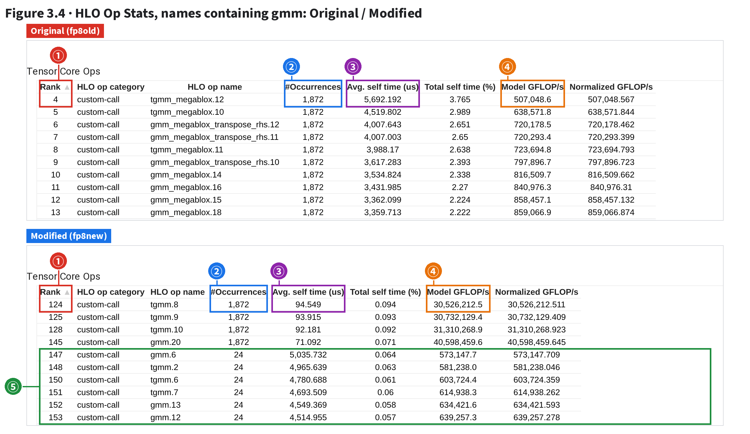
Filter for gmm, with the two runs stacked:

| # | What | On the page (boxes at the on-page text) |
|---|---|---|
| ① | Rank | Rank of the first expert matmul: 4 in the original (tgmm_megablox.12), 124 modified (tgmm.8) |
| ② | #Occurrences | 1,872 in both = 78 iterations × 3 steps × 8 TensorCores (4 chips on this host): not one call fewer |
| ③ | Avg. self time | 5,692.2 µs → 94.5 µs per call (first row) |
| ④ | Model GFLOP/s | 507,049 → 30,526,213 GFLOP/s (507 TFLOP/s → 30.5 PFLOP/s): same numerator (self-reported FLOPs), the time 60× smaller |
| ⑤ | The few that run once per step | Modified: gmm.6, tgmm.2… appear 24 times (once per step per core, outside the 78-iteration loop), 4.2–5.0 ms and 573–686 TFLOP/s per call. Not shrunk (outputs shaped like bf16[192,1536,4096], all 192 experts): the MTP layer (§4.6) |
Same count (②): every iteration made its calls. Time per call fell from 5,692 µs to 94.5 µs; Model GFLOP/s, self-reported FLOPs ÷ time per call, rose 60× with it, to 30.5M GFLOP/s (30.5 PFLOP/s). Not all shrank: the once-per-step calls (⑤, outside the loop) still take 4.2–5.0 ms at 573–686 TFLOP/s, the same order of magnitude as the original's kernels of the same kind. They are the MTP layer's expert matmuls (multi-token prediction: an extra layer after the trunk that predicts one more token), whose weights are gathered by a separate path (§4.6).
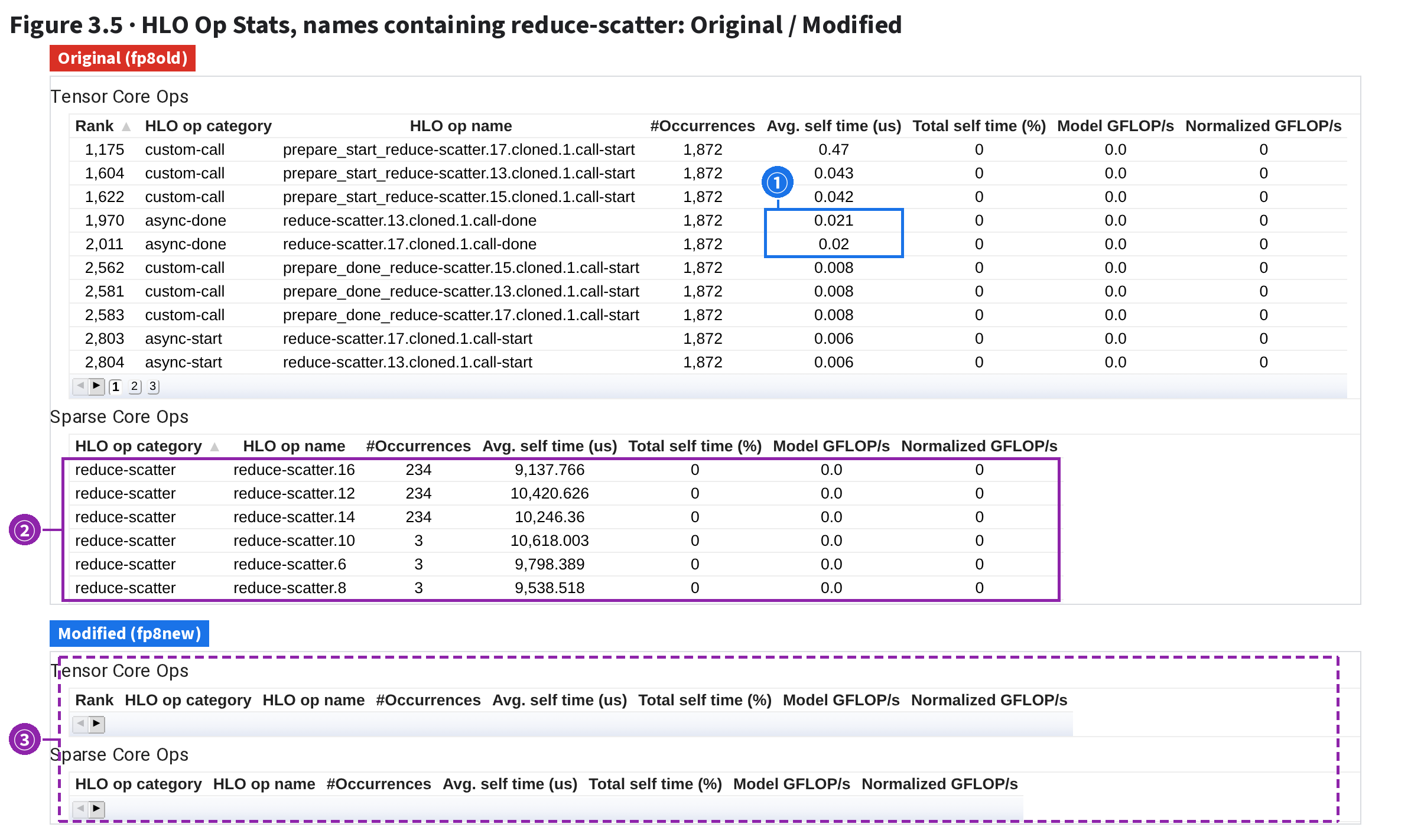
A SparseCore table sits at the bottom of the page; filter for reduce-scatter:

| # | What | On the page (boxes at the on-page text) |
|---|---|---|
| ① | Dones on the TensorCore | Original TensorCore table: reduce-scatter.13/17….call-done average 0.021/0.020 ms per call. When the TensorCore reaches the done, the SparseCore is long finished: these collectives were already hidden under compute |
| ② | Execution on the SparseCore | Original SparseCore table, 6 reduce-scatters: .16/.12/.14 run 234 times each (78 iterations × 3 steps; one SparseCore only), 9.1–10.4 ms per call, 2,354.7 ms per step in all (trace, by type: 2,354.0); .10/.6/.8 3 times each (once per step, outside the loop) |
| ③ | Modified: both tables empty | Same filter: no reduce-scatter in either table. The expert gradients were never scattered back |
The Sparse Core Ops table records each instruction the SparseCore executes: the very collectives of the §2 trace. The original has six expert-gradient reduce-scatters, three in the loop (78 per step each, 9.1–10.4 ms per call) and three outside (one per step, 9.5–10.6 ms), 2,354.7 ms per step; the modified run has none in either table. Their dones on the original's TensorCore take only 0.02 ms: already hidden under compute (as §2.5 concluded), so losing them saves the TensorCore almost nothing; the savings are mostly expert matmuls.
= at its right for “Contains”, and gmm then catches gmm and tgmm.hlo_stats (HLO Op Stats under Tools on the start page). In Visible Columns above the table, tick only Rank, HLO op category, HLO op name, #Occurrences, Avg. self time (us), Total self time (%), Model GFLOP/s, Normalized GFLOP/s: Program id is a program fingerprint, and HLO op text runs to several hundred characters a row.= in the HLO op name box for “Contains” and enter gmm. Figure 3.5: same with reduce-scatter; scroll down to Sparse Core Ops.⭐ The step is 3,916.1 ms shorter: expert matmuls 3,570.5 ms less, waiting on dones 485 ms less; elsewhere actually took a little more. If each device computed only its own 3/192, the skipped matmuls should save 3,611 ms. Both ends match.
| TPU:0 median step (ms) | Original | Modified | Saved |
|---|---|---|---|
| One step | 11,758.2 | 7,842.1 | 3,916.1 |
| custom-call | 6,545.0 | 2,971.9 | 3,573.1 |
| of which expert matmuls (gmm/tgmm, 957 ops) | 3,668.8 | 98.3 | 3,570.5 |
| Waiting on dones (collectives, gather_offload, other async transfers) | 969.0 | 483.6 | 485.4 |
| Elementwise ops (non-fusion elementwise) | 155.9 | 22.2 | 133.7 |
| loop fusion | 2,166.5 | 2,442.4 | −275.9 |
| Other categories | −0.2 | ||
One end is time: 91% of the 3,916.1 ms saved is expert matmuls (same 957 ops, 97% less time). The other end is work: 192 experts over the FSDP group's 64 devices is 3 per device. If each modified device computed only its own 3, it skipped 189/192 of the work (whether it did must be checked in the HLO). All 192 took the original 3,668.8 ms; if time scales with expert count, the skipped part is worth 3,668.8 × 189/192 = 3,611.5 ms [inferred], vs an actual 3,570.5 ms: 1% off.
The SparseCore's skipped gradient scatter and weight gather (2,354 ms of reduce-scatter, about 1,200 ms of all-gather) aren't in this table: they overlapped TensorCore compute anyway and show up only as the 485 ms less waiting (119 ms of it collective dones, §2.5; the rest other async dones such as gather_offload, not split further). Loop fusion actually takes 276 ms more in the modified run. Less work, yet a category grew? Note it; §4.6 finds the cause in the HLO.
⭐ 90% of the 3.9 seconds saved is expert matmuls never computed.
⭐ One profile's step takes 375 s, 31.9× the original. Op Profile's first row names it: custom-call, 98.49% of time at 0.94% utilization. Op Stats' top 10 are all expert matmuls at 0.37–0.42 s per call.

| # | What | On the page (boxes at the on-page text) |
|---|---|---|
| ① | Overall FLOPS utilization | 0.62% (original: 20.20%) |
| ② | The custom-call category | TIME 98.49%, WASTED 97.56%: the 375-second step is almost all Pallas kernels |
| ③ | custom-call FLOPS | 0.94% (original: 53.39%): tens of times the time, same booked FLOPs (all three FP8 runs: 3,966 TFLOP per step per core) |
| ④ | Top 10 all expert matmuls | tgmm_megablox/gmm_megablox/gmm_megablox_transpose_rhs fill the top 10, still 1,872 calls each |
| ⑤ | Time per call | 367,386–418,121 µs (0.37–0.42 s) per call vs 3.4–5.7 ms in the original: about 109× slower (gmm_megablox.16: 373,915.2 ÷ 3,432.0 µs). Model GFLOP/s only 7,719 |
This is the original recipe rerun with a byte-identical config; that run just didn't inject the expert-matmul tile sizes, so every kernel used the default 128 × 128 × 128.
A tile is the block of matrix a kernel loads on-chip and computes at once. Too small, and movement and scheduling overhead swamp the math, idling most compute. The compiled program sets all these kernels to tile 128×128×128 (7,511 sites); the original uses sizes like 512×2048×1536.
Each expert matmul ran about 109× slower (⑤), the step 31.9×.
Two cases, one page. Modified: custom-call has little time at over 100% utilization. More work booked than done: find who skipped it. 375-second run: custom-call has all the time at under 1%. Nothing missing, just extremely slow: check the kernel config. One reading for both: put a category's time share next to its utilization, then expand to the kernel.
| Per step, per TensorCore | Original | Modified | 375-second run |
|---|---|---|---|
| custom-call booked FLOPs (TFLOP) | 3,966.1 | 3,966.1 | 3,966.1 |
| custom-call measured time (ms) | 6,541.8 | 2,972.8 | 369,525.1 |
| Utilization on the page | 53.39% | 117.45% | 0.94% |
One gmm_megablox.16/gmm.27: time per call | 3,431.1 µs | 48.6 µs | 373,755 µs |
| self-reported 2.886 TFLOP ÷ that time | 841 TFLOP/s | 59,387 TFLOP/s | 7.7 TFLOP/s |
All three book the same FLOPs; only the denominator differs: absurdly shrunk when modified, ballooned in the 375-second run.
fp8tk: Op Profile as in §3.1 (Group by = Category); Op Stats as in §3.3, unfiltered, TensorCore table top 10.⭐ The modified recipe neither gathers the 192 experts' weights nor scatters their gradients: memory should fall a lot. Did it?
§3.4 settled time; memory is a separate ledger. The original recipe must gather all 192 experts' weights before computing, and the backward pass yields a full 192-expert gradient that must be held until scattered back to the devices:
one bf16[192,4096,1536] block is 2,304 MiB (192 × 4,096 × 1,536 × 2 bytes). If the modified recipe truly skips both, these blocks should be gone and the peak several GiB lower.
XProf shows memory on two pages: Memory Profile, the runtime allocator's view, over time; Memory Viewer, the compiler's allocation plan for one program, over instruction index. Step through the recording first:
| Stop | Page and action | What you read |
|---|---|---|
| 1 | fp8old Memory Profile, as it opens | Capacity 94.74 GiB, window peak 93.28 GiB, peak time 1.4 ms; Stack 49.39 + Heap 43.89 + Free 1.46; all three lines flat |
| 2 | Set the Memory ID drop-down to 1 | Peak time 23,606.7 ms, 93.23 GiB; the default 0 (TPU:0) logs 128 extra small allocations, putting its peak at the window's start |
| 3 | Enter 23606.7 in “HLO's at time” above HLO Modules | Only jit_train_step is running (8 rows = 8 TensorCores, 7 on screen); Memory Breakdown Table: stack 49.387, unused preallocated 43.846 GiB |
| 4 | Switch to Memory Viewer | Default module jit_add, peak 0.00 MiB: switch modules first |
| 5 | Pick jit_train_step in the Hlo Modules drop-down | Peak 91,766.56 MiB; entry parameters 44,533.22; temporaries 47,230.39; x-axis is Program Order. The header's Module Name stays jit_add (not refreshed in this version); trust the drop-down |
| 6 | Scroll down to HLO Ops at Peak; under by Buffer Size, hover the widest bar | A 5,688 MiB f32[3,79,…]: a parameter or its nu (6 equal-width bars, reordered each time the page opens) |
| 7 | Hover the second bar | The other kind: nu, or an expert weight under state['model'] |
| 8 | Hover the half-width bars | mu in bf16, 2,844 MiB; params + nu + mu = 44,533 MiB |
| 9 | Next bar of the same width | bitcast_convert_fusion.11: Temporary, no Framework Op, a bf16 weight copy the compiler inserted |
| 10 | Further right, the 2,304 MiB bars | tgmm_megablox.10, bf16[192,4096,1536]: this layer's full gradient for all 192 experts. 5 blocks of this shape, 11.25 GiB: 3 from this layer, 2 from the MTP layer's expert-gradient all-reduce |
| 11 | Same page, fp8new | Peak 91,597.20 MiB; the three widest are now the output-head logits bf16[7,4096,120832]; no [192,…] gradients left in the peak list |
| 12 | Same page, bf16old | Parameter param.329 (wo) f32[192,79,1536,32]: all 192 experts present, the 4,096 dimension cut to 32; entry parameters 22,271 MiB, half of FP8 |
Full video: topic07-xrec-mem.en.mp4 (the poster is the stop-10 frame, png).

| # | What | What the page shows (boxes follow page text and bars) |
|---|---|---|
| ① | Memory ID | Defaults to 0 (TPU:0), which logs 128 extra small allocations (#Allocation 196 vs 68), so its peak lands at 1.4 ms, the window's start; the training step doesn't begin until 380 ms. Switch to 1; Memory IDs 1–7 all match |
| ② | Window peak | 93.23 GiB (93.28 on Memory ID 0) against a capacity of 94.74 GiB: only 1.50 GiB left |
| ③ | Peak time | 23,606.7 ms, inside the profile's second step |
| ④ | Stack/Heap/Free | 49.39 + 43.85 + 1.50 = 94.74 GiB. Stack is workspace reserved in one block at launch; Heap is arrays kept across steps (⑨) |
| ⑤ | Timeline | All three lines are nearly flat: memory is allocated in one block at launch, so the allocator never sees the program's ups and downs. This chart can show only peak and headroom |
| ⑥ | HLO's at time | Enter the peak time, 23606.7; the module table keeps only the program then running |
| ⑦ | Running at that moment | Only jit_train_step. 8 rows (8 TensorCores), 7 on screen; scroll the table for TPU:6. It spans about 12,213–23,970 ms: the peak belongs to the training step |
| ⑧ | stack | First entry in the Memory Breakdown Table: 49.387 GiB, the Stack from ④ |
| ⑨ | unused preallocated | Second entry, “unused preallocated device memory”, 43.846 GiB, allocated before the profile started. Despite the name, it is within 0.36 GiB of Memory Viewer's entry parameters (parameters + optimizer state, 44,533 MiB = 43.49 GiB) [inferred: the parameters and optimizer state were allocated before the window opened, and the allocator records them as one block] |
The lines stay flat because the training program reserves its whole workspace in one block at launch (Stack), and parameters and optimizer state predate the profile (Heap).
The peak time is just the moment a 512-byte allocation landed: enter it in HLO's at time, confirm jit_train_step is running, and move on.
The original peaks at 93.23 GiB, the modified run at 91.57 GiB: only 1.66 GiB less. To see what holds it, open this program in Memory Viewer.

| # | What | What the page shows (boxes follow page text and bars) |
|---|---|---|
| ① | Peak | A 91,766.56 MiB (89.6 GiB), B 91,597.20, C 88,401.89 MiB. This program only, from the compile-time plan, so it is below Memory Profile's runtime peak (§3.6 text; fold “Where the two peaks differ”). The header's Module Name still says jit_add: open-source 2.23.1 doesn't refresh it after a module switch; trust jit_train_step in the left-panel drop-down |
| ② | Entry parameters | A and B both 44,533.22 MiB, C 22,271.03 MiB: BF16 is almost exactly half, 4.4 MiB over (fold “Why BF16's entry parameters are half of FP8's”) |
| ③ | Temporaries | Temporaries alive at the peak: A 47,230.39, B 47,061.12, C 66,127.62 MiB. The curve's x-axis is Program Order (instruction index), not time; the green band is the peak span: instructions 3,204–3,319 in A, earlier in B |
The header has three numbers: the peak; entry parameters, arrays passed in at program start (parameters, optimizer state, this step's data); temporaries, buffers allocated during the run and freed after use (activations, gathered weights, gradients not yet scattered). The green band (peak span) sits at instructions 3,204–3,319 in the original, earlier in the modified run (near instruction 1,687). The two peaks differ by only 169 MiB, against an estimated saving of several GiB, and the peak has moved. See what is live there.
![Figure 3.9 · Largest buffers at the peak: by Buffer Size (equal-width bars boxed together). ① Params ×3 + nu ×3 (f32); ② mu ×3 + bf16 weight copies ×3 + grad accumulators ×3; ③ [192,…] expert grads ×5 (3 from the loop + 2 from MTP); ④ Logits ×3; ⑤ Params ×3 + nu ×3 (f32); ⑥ mu ×3 + bf16 weight copies ×3; ⑦ MTP layer's gathered [192,…] ×3; ⑧ Logits ×3; ⑨ Sorted tokens ×2; ⑩ Params ×3 + nu ×3 (f32); ⑪ Gathered [192,…] ×3](img/topic07-39-membysize.en.png?v=f7e5da7f)
| # | What | What the page shows (boxes follow page text and bars) |
|---|---|---|
| ① | Params ×3 + nu ×3 (f32) | FP8 Original: 6 bars × 5,688 MiB. param.467, param.393, param.471, param.391, param.469, param.392 |
| ② | mu ×3 + bf16 weight copies ×3 + grad accumulators ×3 | FP8 Original: 9 bars × 2,844 MiB. bitcast_convert_fusion.11, broadcast.4714.clone, broadcast.4714.clone2, broadcast_in_dim.1367.clone, param.468, param.466 |
| ③ | [192,…] expert grads ×5 (3 from the loop + 2 from MTP) | FP8 Original: 5 bars × 2,304 MiB. all-reduce.358, tgmm_megablox.11, tgmm_megablox.10, tgmm_megablox.12, all-reduce.354 |
| ④ | Logits ×3 | FP8 Modified: 3 bars × 6,608 MiB. multiply_convert_fusion.1, fusion.1176{1}, select_reduce_fusion.3{1} |
| ⑤ | Params ×3 + nu ×3 (f32) | FP8 Modified: 6 bars × 5,688 MiB. param.619, param.620, param.695, param.697, param.699, param.621 |
| ⑥ | mu ×3 + bf16 weight copies ×3 | FP8 Modified: 6 bars × 2,844 MiB. copy.2313, copy.2312, copy.2311, param.694, param.698, param.696 |
| ⑦ | MTP layer's gathered [192,…] ×3 | FP8 Modified: 3 bars × 2,304 MiB. all-gather.537, all-gather.539, all-gather.538 |
| ⑧ | Logits ×3 | BF16 Original: 3 bars × 11,328 MiB. multiply_convert_fusion.1, select_reduce_fusion.2{1}, fusion.1248{1} |
| ⑨ | Sorted tokens ×2 | BF16 Original: 2 bars × 3,072 MiB. gather_offload_custom_fusion.81, gather_offload_custom_fusion.79 |
| ⑩ | Params ×3 + nu ×3 (f32) | BF16 Original: 6 bars × 2,844 MiB. param.403, param.327, param.329, param.328, param.405, param.407 |
| ⑪ | Gathered [192,…] ×3 | BF16 Original: 3 bars × 2,304 MiB. all-gather.578, all-gather.577, copy.1476.args_refs_4_.args_refs_4_ |
Scroll down to HLO Ops at Peak Memory Allocation Time: one bar per buffer live at the peak, widest first under by Buffer Size. Hover a bar for its name, size, shape and Framework Op (the name path JAX recorded) in the left panel. One by one, they fall into three kinds:
[3,79,…] is the 3 experts each device holds. The half-width bars are mu, stored as bf16. Params 17,813 + nu 17,813 + mu 8,906.5 = 44,533 MiB, the header's entry parameters.bitcast_convert_fusion.11 and the like have no Framework Op field in the left panel at all. In the HLO it turns the f32 parameter into re-laid-out bf16: a weight copy the compiler inserted for the computation. It has no line in the code; no code change removes it. Its width group also has three bf16[79,3,…] broadcasts (“grad accumulators” in Figure 3.9), 79 layers × 3 experts per device, op_name in the backward transpose(jvp()). The HLO zero-fills them ahead of the backward loop (while); each pass writes this layer's 3 expert weight gradients into its slot (dynamic-update-slice). Filled as backward runs, they live through the whole loop.tgmm_megablox.10/11/12, 2,304 MiB each, bf16[192,4096,1536], Framework Op with transpose(jvp())/while/body. In the backward loop body: this layer's full weight gradient for all 192 experts, not yet reduce-scattered back to 3: the drhs before psum_scatter in §4.5's code ④ (the expert-weight gradient: in the matmul lhs × rhs, rhs is the weight, and d marks a gradient).
Two more of this shape, all-reduce.354/358: MTP-layer expert gradients summed over all 128 devices outside the loop, kept until the optimizer update. Five blocks, 11.25 GiB; the peak lands while they are live.In B (modified), the three widest are now bf16[7,4096,120832], 6,608 MiB each: the output head's logits, a score per vocabulary entry per position (7 sequences per device × 4,096 tokens × 120,832 entries).
None of the loop's 3 [192,…] gradient blocks appear in its peak list: tgmm emits [3,…] directly; this layer's gradient scatter is gone.
The MTP all-reduce remains (all-reduce.364/366/368), just not at the peak. The 3 [192,…] left in the list are the MTP layer's gathered weights, op_name convert_element_type (again in §4.2, §4.6).
⭐ Those blocks did vanish, but the peak is just the top moment, now the output-head logits, not the backward span: only 169 MiB lower. Memory and time agree: the loop gathers and scatters nothing.
| Block | Size | Contents | How checked |
|---|---|---|---|
| Heap | 44,899 MiB (43.85 GiB) | Arrays that persist across steps, allocated before the profile started (unused preallocated device memory in the Memory Breakdown Table) | Memory Profile |
| ├ Expert and other weights (f32) | 17,813.0 MiB | state['model']…, 44 blocks | Memory Viewer entry parameters, split by Framework Op |
| ├ Adam second moment nu (f32) | 17,813.0 MiB | state['optimizer']…['nu']… | Same |
| ├ Adam first moment mu (bf16) | 8,906.5 MiB | …['mu']…, stored as bf16, hence half | Same |
| ├ Data batch and step count | 0.6 MiB | data['inputs'] etc. | Same |
| └ Unaccounted | 366 MiB | Heap beyond the entry parameters; the allocator records Heap as one block, with no per-buffer breakdown | not checked |
| Stack | 50,573 MiB (49.39 GiB) | Workspace reserved in one block at program start: activations, temporarily gathered weights, gradients not yet scattered, compiler-inserted copies, logits | Memory Profile |
| ├ Compile-time temporary area (incl. fragmentation) | 49,473.0 MiB | Fourth line of the Memory Viewer header, “HLO lifetime temporary variables with fragmentation” | Memory Viewer |
| └ Unaccounted | 1,100 MiB | Stack beyond the compile-time temporary area; reserved as one block at runtime, with only a total in the profile | not checked |
ici_fsdp_parallelism=64 × ici_data_parallelism=2: parameters are cut into 64 shards, each stored on 2 devices, so each device holds 1/64 and the expert weights have shape [3,79,4096,1536] (sharded along the expert dimension).ici_fsdp_parallelism=-1: 128 devices, 128 shards, 1/128 each. Expert weights are f32: wi_0/wi_1 are [192,79,32,1536] and wo is [192,79,1536,32] (param.329, hovered at stop 12, is wo; all three are split along the 4,096 dimension, 32 per shard: what Section 5 calls the expert dimension left unsharded). Entry parameters: 22,271 MiB, almost exactly half of FP8 (4.4 MiB over).http://127.0.0.1:6311/?run=fp8old/2026_08_15_03_57_28&tag=memory_profile&host=gke-node-1; set Memory ID (top right) to 1; enter the peak time in “HLO's at time (ms)” above the HLO Modules table and press Enter.http://127.0.0.1:6311/?run=fp8old/2026_08_15_03_57_28&tag=memory_viewer&host=gke-node-1; in the left panel, pick jit_train_step(…) from the Hlo Modules drop-down and wait a dozen or so seconds for the chart; scroll down to HLO Ops at Peak Memory Allocation Time and hover a bar under by Buffer Size for details in the left panel (long; scroll the panel).fp8new/bf16old.⭐ Time and memory both add up: 90% of the missing 3.9 s is expert matmuls never computed. But a profile records only what happened; why each device got only 3 experts takes the HLO and the code.
Section 3 balanced the books: 90% of the missing 3.9 s is expert matmuls never computed. Which part of the program is gone? A profile records only what happened, not what didn't. To see what should be there, read the program itself: the final HLO the compiler hands the chip.
⭐ HLO is your JAX program after XLA has partitioned, fused and scheduled it: one instruction per line, a shape on every value. Every slice name in the trace is an HLO instruction name.
HLO (the IR of XLA's High Level Optimizer) is the compiler's internal program form. You write a train_step; the compiler splits it across 64 devices, fuses elementwise chains into fusions,
inserts collectives and fixes the order, giving the final HLO, one line like this per instruction:
name = type[shape] opcode(operands, …), attributes…
gmm.27 = bf16[229376,1536] custom-call(…, get-tuple-element.14549, …), custom_call_target="tpu_custom_call"
The second line is the gmm.27 from Sections 2 and 3: a bf16 output of 229,376 × 1,536, and custom-call means a call into an external kernel (the Pallas expert matmul).
The trace tells you when each instruction runs and for how long; the HLO, what goes in and out and which instructions exist at all, including ones never generated, which no profile shows.
| Where | How | Good for |
|---|---|---|
| Open-source XProf pages | Graph Viewer: pick a module and an instruction to draw what feeds it and what it feeds (§4.3). Op Stats' HLO op text column: the full text | One instruction's inputs and outputs, in the browser |
| From the profile files | The profile stores the whole compiled HLO (HloProto) in xplane.pb; its directory also holds a <module>.hlo_proto.pb per module. Parse with XLA's hlo.proto to get text | Whole-program counts: how many of a kind, in which loop (all of this section's counts) |
| XLA dump at compile time | Rerun with XLA_FLAGS="--xla_dump_to=DIR --xla_dump_hlo_as_text"; *after_optimizations.txt is the final HLO | No profile yet, or to see each compiler pass (recompile) |
{3,2,0,1:T(32,128)(4,1)}), a whole backend_config JSON blob, and long names stacked layer upon layer.name = type[shape] opcode(operands), tagging each line with its op_name (JAX's name path, §4.5). The modified step's HLO text drops from 8.4M to 3.8M bytes, the original's from 9.6M to 6.8M; a loop body becomes a few hundred readable lines.Click a slice in Trace Viewer and its raw HLO appears under Start Stack Trace in Details; Graph Viewer nodes and Op Stats' HLO op text column show the same text. Below is the original recipe's gmm_megablox.16 line (same screenshot as recording stop 2 in §4.3):

| # | What | How to read it (boxes follow the text on the page) |
|---|---|---|
| ① | name = result opcode(operands…), attributes… | One instruction per line. Drop the % and the name is the slice name in Trace Viewer (leave the % out in Find Events) |
| ② | type + shape | bf16[229376,1536]: an output of 229,376 rows × 1,536 columns. 229,376 = 7 sequences per device × 4,096 tokens × 8 experts per token (the §0.2 config); f8e4m3fn is FP8 (4 exponent bits, 3 mantissa bits) |
| ③ | {1,0: dimension order in memory | minor_to_major: the first number is the dimension that varies fastest in memory. {1,0} is row-major (openxla.org/xla/shapes) |
| ④ | :T(16,128)(2,1): tiling | tiling: tile by 16×128 first, then (2,1) packs 2 adjacent bf16 values in a column into one 32-bit word (FP8 uses (4,1), 4 per word). The official tiled_layout page gives (8,128)(2,1) as typical for bf16; the HLO measured in this course has 16×128, and 32×128 for FP8. Go by the HLO |
| ⑤ | custom-call + target | custom-call = call an external kernel; custom_call_target="tpu_custom_call" = a Pallas kernel on TPU (JAX's public source, tpu_custom_call.py, uses exactly this name) |
| ⑥ | one operand: type %name | Each operand in the parentheses is written “type name”, in the order of the 0, 1, 2… on Graph Viewer's edges: s32[193]{0:T(256)} %copy-done.141 is operand 1 (recording stop 8 ①) |
| ⑦ | weights: 192 experts | Operand 7, f8e4m3fn[192,4096,1536]{2,1,0:T(32,128)(4,1)}: FP8, 192 experts, 32×128 tiles. This one number is what Section 4 is hunting for |
| ⑧ | suffix after the operand name | .args_refs_4_.qvalue: which kernel argument this data feeds (the quantized value of argument 4) [inferred from the name; we didn't check the source that builds it] |
| ⑨ | per-operand layout constraints | operand_layout_constraints={…}: the layout the kernel requires for each operand, in the same order as the parentheses; s32[193] and f8e4m3fn[192,4096,1536] appear here again |
| ⑩ | kernel-reported metadata | kernel_metadata carries this kernel's tile: tile_m 512, tile_k 2048, tile_n 1536, the tile set the original recipe injects (§0.2 fold: the tiles injected at runtime) |
For a collective, read three more attributes (§4.2's all-gather.573; all-gather.580, Section 5's BF16 expert-weight gather):
| Attribute | Example | How to read it |
|---|---|---|
replica_groups | mesh[…'fsdp'=64…] {'fsdp'} | Which devices form a group: only the fsdp axis is named, so 64 devices. The group size is the number of shards the tensor is split into |
dimensions | {1} (573), {2} (580) | The dimension to concatenate along: 573 concatenates the expert dimension, [1,3,…] → [1,192,…]; 580 the 4096 dimension, [1,192,32,1536] → [1,192,4096,1536] |
is_spmd_generated="true" | 580 has it, 573 doesn't | Literally, generated during SPMD partitioning: the compiler inserted it to match the weights' sharding, so you won't find this all_gather in the code. 573 lacks it: it was written by hand inside a shard_map in the code (① in §4.5; its op_name also ends in shard_map/all_gather) |
*-done among the operands (which communication it waits on) → layout and tiling last (if you suspect padding or a relayout).⭐ Counted line by line: the original has 12 all-gathers taking expert weights from this device's 3 to 192, and 6 reduce-scatters taking gradients from 192 back to 3. The modified run has none of these 18.
| Count in the final HLO | Original | Modified | Reading |
|---|---|---|---|
| all-gather/reduce-scatter/all-reduce (all) | 92/6/36 | 82/0/36 | all-reduce unchanged, 10 fewer all-gathers, no reduce-scatter left |
Expert-weight gathers: f8e4m3fn [1,3,…] → [1,192,…] | 12 | 0 | 3 in the forward loop, 3 in the backward (regathered for recompute), 6 outside (the peeled-out layer) |
Expert-gradient scatters: bf16 [192,…] → [3,…] | 6 | 0 | 3 in the backward loop, 3 outside; the loop's 3 are Section 2's 9–10 ms reduce-scatters on the SparseCore |
Each MoE layer has three expert matrices (two up-projections, one down), hence the threes. The total (92 → 82) only says something is gone; counting by shape says what: expert weights and gradients. Here is the original's forward loop gathering gmm's first weight matrix (stripped; elided operands as …):
── Original · forward loop body
all-gather.574.cloned.1.call-start = ((f8e4m3fn[1,3,4096,1536], token[]), f8e4m3fn[1,192,4096,1536])
async-start(fusion.1669, …)
└ all-gather.573 = f8e4m3fn[1,192,4096,1536] all-gather(param_0.13420),
replica_groups=mesh[…'fsdp'=64…] {'fsdp'}, dimensions={1}
all-gather.574.cloned.1.call-done = f8e4m3fn[1,192,4096,1536] async-done(all-gather.574.cloned.1.call-start)
bitcast.3183 = f8e4m3fn[192,4096,1536] bitcast(all-gather.574.cloned.1.call-done)
gmm_megablox.16 = bf16[229376,1536] custom-call(…, clamp_convert_fusion.165, …, bitcast.3183, …) # weights: 192 experts
── Modified · forward loop body
fusion.1642 = (f8e4m3fn[3,4096,1536], f8e4m3fn[3,4096,1536]) fusion(…), kind=kLoop # local 3 experts → FP8
gmm.27 = bf16[229376,1536] custom-call(…, clamp_convert_fusion.165, …, get-tuple-element.14549, …)
# weights: f8e4m3fn[3,4096,1536]
── Backward loop body: Original / Modified
tgmm_megablox.10 = bf16[192,4096,1536] custom-call(…)
→ reduce-scatter.13….call-start = ((bf16[192,4096,1536], …), bf16[3,4096,1536])
tgmm.8 = bf16[3,4096,1536] custom-call(…) (no reduce-scatter after it)
192 ÷ 64 = 3 is right there in the first line: the async-start takes this device's [1,3,4096,1536] and outputs [1,192,4096,1536].
Inside, all-gather.573 does the work: it groups only along the 'fsdp'=64 axis (64 devices) and concatenates along dimension 1, 3 × 64 = 192.
This is Section 2's all-gather on the SparseCore row; async_execution_thread="sparsecore" in the HLO sends it there.
In the modified run, gmm.27's weights, [3,4096,1536], come straight from a fusion that only quantizes; nothing is gathered in between.
Section 1 said the original quantizes to FP8 before gathering. Did the modified run just move that step? Trace fusion.1669 (original) and fusion.1642 (modified) up to the parameters:
📌 ① Expert parameters (fp8old param.391, fp8new param.619/620) f32[3,79,4096,1536], sharding devices=[64,1,1,1,2] … last_tile_dim_replicate; ② converted to bf16 before the loop: fp8old bitcast_convert_fusion.11 (the fusion body is just convert f32→bf16, in ENTRY, once per step), fp8new copy.2312/.2313 (an f32 → bf16 copy).
📌 ③④ In the loop body: fp8old fusion.1669, fp8new fusion.1642 (two matrices at once), both dynamic-slice one layer → multiply(×2) → clamp(−448, 448) → convert f8e4m3fn. 2 = 448 ÷ 224: the config sets weight_quantization_calibration_method=fixed,-224,224, and the largest finite value f8e4m3fn can represent is 448 [our derivation].
📌 ⑤⑥ fp8old: fusion.1669 → all-gather.574 (wrapping all-gather.573, {'fsdp'}, 64 shards, dimensions={1}) → bitcast → operand 7 of gmm_megablox.16; 2.380 ms on the SparseCore in layer 40's forward pass. fp8new: fusion.1642's output is operand 7 of gmm.27, [3,4096,1536]. What crosses the network is the other 63 shards, 1,152 × 63/64 ≈ 1,134 MiB.
📌 ⑦ “If gathered as bf16”: bf16[192,4096,1536] = 2,415,919,104 B. A ready-made example in the same program: the MTP layer's expert weights are gathered in bf16 by compiler-inserted all-gathers (fp8new all-gather.537/538/539). Token activations: both runs use clamp_convert_fusion.165 → f8e4m3fn[229376,4096] (gmm operand 5), config act_quantization_calibration_method=fixed,-224,224.
| # | Step | Original | Modified |
|---|---|---|---|
| ① | f32 master (3 local experts × 79 layers) | f32[3,79,4096,1536], 5,688 MiB, same in both | |
| ② | To bf16 before the loop, once a step | bf16[79,3,4096,1536], 2,844 MiB | |
| ③ | This layer sliced out in the loop | bf16[1,3,4096,1536], 36 MiB | |
| ④ | Quantize: ×2, clamp to ±448, to FP8 | f8e4m3fn[1,3,4096,1536], 18 MiB; the same four ops and two constants | |
| ⑤ | After quantizing | Gathers all 64 FP8 shards; 2.38 ms on SparseCore, layer 40 forward | No gather |
| ⑥ | Weights the kernel receives | f8e4m3fn[192,4096,1536], 1,152 MiB | f8e4m3fn[3,4096,1536], 18 MiB |
| ⑦ | Bytes gathered in this step | 1,152 MiB (2,304 MiB if gathered as bf16 first) | 0 |
Quantization is identical to the character; the 2 is 448 ÷ 224 (the config's weight quantization range is ±224; FP8's maximum is 448). The original does quantize first, so it gathers FP8, half the bytes of bf16; the modified recipe didn't move it, only dropped the all-gather after it.
[4096,192] weight (gathered along the 4096 dimension), and bf16 versions of the three expert matrices of the MTP layer (multi-token prediction, the one layer beyond the 80-layer trunk), bf16[3,4096,1536] → [192,4096,1536].convert_element_type rather than shard_map/all_gather: the compiler inserted them to match the weights' sharding, not the gathering lines in the code (all three of these all-gathers carry is_spmd_generated=true; the §4.1 fold explains the attribute). So in both programs the MTP layer gathers all 192 experts before computing (more in §4.5).[3,1,4096,1536] → [192,1,4096,1536]. So the table counts 12 by shape but 10 by instruction.⭐ Original gmm_megablox.16’s weight, traced up: this device’s [1,3,…] → all-gather over 64 devices → [192,4096,1536]. Modified gmm.27’s weight: this device’s [3,4096,1536]. Both kernels get a 192-group token table.
Graph Viewer (an XProf page) draws one center instruction with its operands upstream and users downstream. Boxes are instructions, arrows data flow; a large titled box is a called sub-computation, a dashed box a node with undrawn inputs. The recording goes from a Trace Viewer slice into Graph Viewer, then up the edges:
| Stop | Action | What you see |
|---|---|---|
| 1 | Click gmm_megablox.16 in the original’s forward layer 40 | Wall Duration 3,425,196 ns; top of the Details right column: a Graph Viewer link |
| 2 | Read Start Stack Trace in Details | HLO text: operands f8e4m3fn[192,4096,1536] and s32[193] (read symbol by symbol in Figure 4.1) |
| 3 | Click the link | XLA Op Name filled but not found: open source ignores the link’s module name; drop-down on jit_add |
| 4 | Pick jit_train_step under XLA Modules | Op name cleared, shortcut buttons on the right; click gmm_megablox.16 (or retype the name and click Search Graph) |
| 5 | The graph appears | Center label too long, so the graph is tiny; Graph Width = levels drawn outward; Save SVG below |
| 6 | Save the SVG and view the whole graph | Red diamond = center; operands above; the large gray box below is the fusion consuming its output; dashed box = inputs not drawn (Graph Width limit) |
| 7 | Zoom into the center node | custom-call, tpu_custom_call, 3.43 ms; operand layouts: f8e4m3fn[192,4096,1536], s32[193]; tile 512 / 2048 / 1536; output bf16[229376,1536] |
| 8 | Read the edge numbers | Operand index: 1 is copy-done.141 (group offsets), 7 is bitcast.3183 (weight) |
| 9 | Follow operand 7 upstream | bitcast ← all-gather.574…call-done ← call-start, with async_execution_thread="sparsecore" |
| 10 | Enter the sub-computation | Actual all-gather.573: this device’s [1,3,…], 'fsdp'=64, dimensions={1} → [1,192,…] |
| 11 | Modified, centered on gmm.27 | Weight f8e4m3fn[3,4096,1536]: operand 7 ← quantization fusion.1642; offsets still s32[193] |
| 12 | Back in Trace Viewer, click gmm.27 | Same HLO line in Details: f8e4m3fn[3,4096,1536], s32[193]; no Graph Viewer needed |
*-done inputs (at the edge, raise Graph Width or re-center) →
Check the HLO text (same line in Details, stop 12).Full video: topic07-xrec-graph.en.mp4 (last frame: png). Figure 4.2: its zoomed views as one static comparison:

| # | What | What the figure shows (boxes follow nodes and text in the Graph Viewer SVG) |
|---|---|---|
| ① | This device’s shard | Parameter 0 = f8e4m3fn[1,3,4096,1536]: this device holds only 3 experts (192 ÷ 64), already FP8 |
| ② | Gathered with whom, along which dimension | all-gather.573’s replica_groups name only one axis, 'fsdp'=64: groups of 64 devices. dimensions={1}: concatenate along dim 1 (experts) |
| ③ | After the gather | Output f8e4m3fn[1,192,4096,1536]: 3 × 64 = 192 experts. Wrapped in an async call (titled box = sub-computation), call-start → call-done outside. This is the all-gather block on the SC0 row |
| ④ | Dropping the extra dimension | bitcast to f8e4m3fn[192,4096,1536]; the arrow goes into gmm_megablox.16 |
| ⑤ | The weight the kernel receives | gmm_megablox.16’s operand shapes list the weight as f8e4m3fn[192,4096,1536]: all 192 experts |
| ⑥ | The row where each token group starts | s32[193]: group offsets for 192 experts (193 = 192 + 1 end). Identical in both: tokens still arrive in 192 groups |
| ⑦ | The weight the Modified kernel receives | gmm.27’s weight is f8e4m3fn[3,4096,1536]: only this device’s 3 |
| ⑧ | Where it comes from | operand 7 = output of fusion.1642, which quantizes this device’s 3 experts to FP8. No all-gather in between; no collective anywhere in the graph |
Up the original kernel’s weight operand runs the whole gather; the modified kernel’s is just this device’s 3 experts, quantized.
Watch ⑥ most: s32[193], offsets for 192 token groups, is the same on both sides. Tokens still arrive in 192 expert groups; the modified run has weights for only 3.
graph_viewer (Graph Viewer under Tools on the home page), run fp8old. In the quick-start list at the bottom, click jit_train_step(…) - gmm_megablox.16 to center on it (modified run: gmm.27). Or type the name into XLA Op Name, set Graph Width to 1, click Search Graph.⭐ Same device, same tokens: the original gathers all 192 experts, computes, then scatters the gradients back; the modified run holds 3 experts and computes only 3 groups.
4.3 leaves a question: the modified kernel multiplies 3 experts’ weights by tokens in 192 groups. Does it fail, or compute something? Both programs on device 0, slowed down:
| Stop | What to watch | What you see |
|---|---|---|
| 1 | Original ① all-gather | The other 189 cells come from the other 63 devices: [1,3,4096,1536] → [1,192,4096,1536] (Figure 4.2 ①–③) |
| 2 | ② gmm | All 192 groups have weights; the right side lights up: 3 gmms per forward layer, 10.1 ms |
| 3 | ③ tgmm + reduce-scatter | Gradients for 192 experts; summed across 64 devices, each keeps only its 3: [192,…] → [3,…] |
| 4 | Modified ① no all-gather | Still holds 3: [3,4096,1536] (Figure 4.2 ⑦⑧) |
| 5 | ② gmm | Only 3 groups’ rows computed, the other 189 written as 0: 3 gmms per layer, 0.11 ms |
| 6 | ③ tgmm | Just 3 experts’ gradients; nothing to scatter |
| 7 | Summary | All shapes legal, no error; 189/192 of the work gone; expert matmuls 3,668.8 → 98.3 ms per step |
Full video: topic07-experts.en.mp4 (last frame: png, same as the first). It shows device 0, which holds exactly experts 0–2; the modified run also computes exactly groups 0–2 [inferred from the code], so on screen they line up one to one. Other devices: the 4.5 fold.
The animation is one device over time. Laid out statically below: how 192 experts split into 64 shards, how many each branch computes:
📌 The split: config num_experts=192, ici_fsdp_parallelism=64, ici_data_parallelism=2 (64 chips × 2 TensorCores = 128 devices). Final HLO: this device’s expert parameter f32[3,79,4096,1536] (3 experts × 79 layers), sharding devices=[64,1,1,1,2] … last_tile_dim_replicate: leading dim 192 cut in order into 64 blocks, each on 2 devices. Device numbers in the figure count along the fsdp axis (0–63); the 2 devices on the data axis hold the same experts.
📌 ① Original all-gather.573: input this device’s [1,3,4096,1536], replica_groups=…{'fsdp'} (64 shards), dimensions={1}, output [1,192,4096,1536] (f8e4m3fn). ② Weight operand: gmm_megablox.16 [192,4096,1536], modified gmm.27 [3,4096,1536]; group offsets s32[193] in both. One forward layer’s 3 gmms: 10.107 → 0.109 ms (layer 40).
📌 ③④ Original tgmm_megablox.10 outputs bf16[192,4096,1536]; reduce-scatter over {'fsdp'} scatters back to [3,4096,1536]; modified tgmm.8 outputs [3,4096,1536] directly. ⑤ Expert-gradient all-reduce (original all-reduce.384, modified .394) runs over {'data'} in both.
📌 Modified, the other 189 groups get 0: public MaxText backend.py builds tables for only this device’s 3 groups, zero-filling the rest (L346–347, L555–561). Which 3 groups device 0 computes is read from code [inferred]; the figure doesn’t number them.
| # | Original | Modified |
|---|---|---|
| ① | The other 63 devices send 3 each, forming [1,192,4096,1536] | No all-gather; it holds just [3,4096,1536] |
| ② | gmm: all 192 groups get weights; layer 40 forward, 3 gmms: 10.1 ms | gmm: only 3 groups have weights, other 189 output 0; 3 gmms: 0.11 ms |
| ③ | Gradients for all 192: bf16[192,…] | Only 3 gradients to begin with: bf16[3,…] |
| ④ | reduce-scatter: sum over 64 shards, each keeps its 3 | None |
| ⑤ | all-reduce: each expert lives on 2 data-axis devices, whose separate gradients are summed (both runs; ⑦ in the Section 2 communication figure) | |
This answers Section 2’s open question: the modified run sums expert gradients only across the 2 data-axis shards; ④, the sum across 64 shards, is gone. Every shape along the way is legal; nothing raises an error.
⭐ An HLO instruction’s op_name names the code branch that ran. Public MaxText has the weight all_gather and gradient psum_scatter only in the tokamax branch; the modified run’s branch calls the kernel directly, with neither.
Every HLO instruction carries an op_name: the name path JAX recorded while tracing, primitive last, enclosing scopes to its left. Their last segments, for the three key instructions:
| Instruction | Last segments of op_name | Which branch |
|---|---|---|
| all-gather.573 (original) | …/while/body/closed_call/shard_map/all_gather | A hand-written jax.lax.all_gather inside shard_map |
| gmm_megablox.16 (original) | …/shard_map/tokamax:{"op":{"__type":"tokamax…PallasMosaicTpuRaggedDot", …}} | Tokamax’s ragged_dot: the use_tokamax_gmm=True branch |
| gmm.27 (modified) | …/shard_map/jit(gmm)/pallas_call | MaxText’s own megablox backend.gmm: the other branch |
Of Section 0’s 13 differing config lines, the only one besides the 12 tile values is use_tokamax_gmm: True → False. The two branches it selects (public repo, version notes in the fold; unrelated lines removed):
# src/maxtext/kernels/megablox/ops.py · _gmm_fwd (forward)
# QAG is only supported for following conditions
if use_tokamax_backend: # L191
if quantization_rule and quantization_rule.bwd_qtype:
if quantization_rule.weight_calibration_method.startswith("fixed") and isinstance(rhs, qpl.QArray):
if weight_gather_axes:
for axis_name, axis_idx in weight_gather_axes:
rhs_qvalue = jax.lax.all_gather(rhs.qvalue, axis_name, axis=axis_idx, tiled=True) # ① L196: gather all 192 experts
rhs = dataclasses.replace(rhs, qvalue=rhs_qvalue)
…
elif use_tokamax_backend:
out = tokamax.ragged_dot(lhs=lhs, rhs=rhs, group_sizes=group_sizes, …) # ② L223 → gmm_megablox.*
else:
out = backend.gmm(lhs, rhs, group_sizes, preferred_element_type, tiling[:3], …) # ③ L235 → gmm.*: rhs still local 3
# same file · _gmm_bwd (backward)
if use_tokamax_backend or use_gmm_v2: # L315
…
drhs = tokamax.ragged_dot_general(lhs=lhs, rhs=drhs_dout, …) # tgmm_megablox.*: [192,4096,1536]
if quantization_rule and quantization_rule.bwd_qtype and weight_gather_axes:
for axis_name, axis_idx in reversed(weight_gather_axes):
drhs = jax.lax.psum_scatter(drhs, axis_name, scatter_dimension=axis_idx, tiled=True) # ④ L392: scatter back to 3 each
else:
dlhs = backend.gmm(dlhs_dout, rhs, group_sizes, …) # ⑤ L394–416: no gather, no scatter
drhs = backend.tgmm(lhs.swapaxes(0, 1), drhs_dout, group_sizes, …) # tgmm.*: [3,4096,1536]
① and ④ are the 4.2 table’s 12 and 6 instructions: forward gather, backward scatter, paired, tokamax branch only. The 3.6 memory peak’s 3 blocks tgmm_megablox.10/11/12 are the drhs ④ scatters. Both branches get weight_gather_axes (in this config, with experts sharded on FSDP and a weight calibration starting with fixed,
the MoE layer passes on “gather along fsdp”), but branch ③⑤ ignores it. Missing forward gather and backward scatter match the profile exactly: all-gather and reduce-scatter both vanish on the SparseCores.
⭐ Why it is silent: backend.gmm already supports devices that own only some expert groups. Seeing 3 weight groups and 192 table groups, it builds metadata and computes rows only for those 3; the rest get 0. Every shape is legal; nothing raises an error.
# src/maxtext/kernels/megablox/backend.py · gmm
num_current_groups = rhs.shape[0] # L346: 3
num_total_groups = group_sizes.shape[0] # L347: 192
… # L374: make_group_metadata(…, num_nonzero_groups=rhs.shape[0]), table for 3 only
if existing_out is None and num_current_groups < num_total_groups: # L555
out = _zero_uninitialized_memory(out, start_group=group_offset[0],
num_nonzero_groups=rhs.shape[0], …) # zero the other rows: jnp.where(valid_mask[:, None], out, 0)
hunyuan3 branch of github.com/yangwhale/maxtext (upstream main plus three commits). Line numbers above: its 1afaa0fb.ops.py and backend.py untouched: both are byte-identical to upstream AI-Hypercomputer/maxtext (formerly google/maxtext) at 188af874 (2026-07-28), same line numbers.ops.py:235 _gmm_fwd (line ③) and backend.py:548 (call_gmm); the two runs’ MoE calls are at moe.py:1504 (tokamax branch) and moe.py:1534 (megablox branch), all matching this version’s line numbers. Call stacks sometimes point to the wrong place; here it agrees with op_name, so it serves as corroboration.group_offset the MoE layer passes to the kernel depends on device index only with ring-of-experts on. Here it is off (use_ring_of_experts=False), so the offset is 0 everywhere: every device computes groups 0–2’s tokens.⭐ Most of the extra loop-fusion time is that zero-fill. The 9 unshrunk expert matmuls outside the loop are the MTP layer, whose experts the compiler gathers.
| Section 3’s puzzle | What HLO and the trace show | Conclusion |
|---|---|---|
| Modified: loop fusion +276 ms | Modified: two extra kinds of loop fusion per layer. Forward broadcast_select_fusion (op_name ends in jit(gmm)/jit(_where)/select_n, output bf16[229376,4096]), 79 per step, 95.1 ms;
backward select_add_fusion, 79 per step, 225.6 ms: three selects (also from jit(gmm)/jit(_where)) plus an add_any summing two inputs’ gradients. In the original that add_any is a standalone elementwise op (135.5 ms per step, under non-fusion elementwise) |
backend.py’s zero-fill (jnp.where): each layer writes 0 to 189/192 of 229,376 rows, once forward, fused with the add backward. The two new fusions total 320.7 ms: ~135.5 ms is the old add, recategorized (meanwhile 3.4’s non-fusion elementwise drops 133.7 ms), and the remaining ~185 ms is the zero-fill itself. Loop fusion as a category grows by only 276 ms because other loop fusions shrink by ~45 ms in total (some up, some down; not traced one by one here) |
| Which layer: 9 unshrunk out-of-loop gmms | The median step has 21 expert matmuls outside the loop. 3 before the forward loop and 9 after the backward loop have while/body in op_name and [3,…] weights and gradients, about 0.05–0.07 ms each (the loop’s peeled layer, shrunk too);
the other 9 lack while/body, have bf16[192,…] gradients, 4.2–5.2 ms each (per kernel, 3 steps on TPU:0; 3.3’s Op Stats averages 8 cores, hence 4.2–5.0). Call stacks pass through multi_token_prediction.py; weight parameter mtp_block/…/MoeBlock_0/wi_0 |
The MTP layer (multi-token prediction, the one layer outside the backbone). The compiler gathers its experts to 192 in bf16 (4.2 fold), bypassing those two lines: nothing skipped, equally slow in both |
⭐ With the gather and scatter moved out of the tokamax branch so both branches share them, a step takes 12.501 s, 6% slower than the original’s 11.761 s. The “50% faster” was all skipped work.
The fix moves ①’s all_gather and ④’s psum_scatter out of the if: gather whenever weight_gather_axes is set; scatter backward whatever was gathered forward.
Post-fix numbers (Hy3 tuning log, TUNING-v7 §3.4.10): 12.501 s per step, 637.0 TFLOP/s per chip; original 11.761 s, 677.0 TFLOP/s.
documented No profile was kept; we can only quote it, not recompute it.
Section 4 confirmed FP8's 3.9 s was skipped work. Conversely, what does a truly faster change look like on the same pages?
No new example needed: the same change (use_tokamax_gmm: True → False plus the same 12 tile values) was also made on the BF16 recipe.
⭐ The BF16 configs differ exactly as the FP8 pair do; one step goes 21,747.2 → 20,693.8 ms, 1,053.4 ms (4.8%) faster.
| Same change | FP8 (§0–4) | BF16 (§5) |
|---|---|---|
| Config diff | use_tokamax_gmm True → False + 12 w{i,o}_tile_* values 1024 → 2048/1536. Both diffs identical (each over the full MaxText config) | |
| One step (TPU:0 median step) | 11,758.2 → 7,842.1 ms (−3,916.1) | 21,747.2 → 20,693.8 ms (−1,053.4) |
| SparseCore all-gather / reduce-scatter (ms/step) | 1,409.3 / 2,354.0 → 205.8 / 0 | 2,522.8 / 2,543.1 → 2,593.7 / 2,606.5 |
| HLO: 192-expert all-gathers / expert-gradient reduce-scatters (count) | 12 / 6 → 0 / 0 | 12 / 6 → 12 / 6 |
| Expert matmuls (gmm family, ms/step) | 3,668.8 → 98.3 (−97%) | 8,183.8 → 7,116.2 (−13%) |
| Op Profile: custom-call FLOPS utilization | 53.39% → 117.45% | 45.57% → 49.62% |
| Op Stats: rank of the first expert matmul | #4 → #124 (out of the top 10) | #4 → #4 (still 7 in the top 10) |
| Expert weights the kernel receives | [192,4096,1536] → [3,4096,1536] | [192,4096,1536] → [192,4096,1536] |
| HBM: largest buffers at peak (Memory Viewer) | This layer's 3 in-loop [192,…] expert-gradient buffers → none left; peak moves to the output head | Same in both: logits + gathered weights of all 192 experts |
In the right column every row is unchanged or barely changed; only the step time and the expert matmuls move. In the left, every row from “SparseCore all-gather” down is an alarm. The next two subsections check the right column in the profile, row by row.
⭐ Backward layer 40 side by side. On the SparseCore, both runs have the 3 all-gathers of the 192 experts and the expert-gradient reduce-scatters, at nearly equal widths. On the TensorCore all 9 expert matmuls are present, 79.11 → 66.89 ms in total.

| # | What | How to tell (names and times from the xplane) |
|---|---|---|
| ① | Expert matmuls ×9 | TC: this layer's 9 expert matmuls (gmm/tgmm) total 79.11 ms 6 boxes in the main figure: gmm_megablox.11+gmm_megablox.12 (at 35,667.665 ms, 8.699/9.627 ms); gmm_megablox_transpose_rhs.8 (at 35,687.634 ms, 8.405 ms); gmm_megablox.13 (at 35,698.274 ms, 7.202 ms); gmm_megablox_transpose_rhs.9+tgmm_megablox.10 (at 35,714.635 ms, 9.961/10.053 ms); gmm_megablox_transpose_rhs.10 (at 35,737.722 ms, 10.414 ms); tgmm_megablox.8+tgmm_megablox.9 (at 35,751.081 ms, 7.827/6.926 ms) |
| ② | All-gather of the 192 experts | SC0: all-gathers 527/529/531 of the 192 experts’ weights: 4.86/4.90/4.86 ms, shapes bf16[1,192,4096,1536] etc. 2 boxes in the main figure: all-gather.527 (at 35,631.171 ms, 4.860 ms); all-gather.529+all-gather.531 (at 35,667.669 ms, 4.899/4.865 ms) |
| ③ | Expert-gradient reduce-scatter | SC0: expert-gradient reduce-scatters 198/200/202: 8.86/8.58/8.16 ms, shapes bf16[192,32,1536] etc. 2 boxes in the main figure: reduce-scatter.198+reduce-scatter.200 (at 35,758.909 ms, 8.855/8.581 ms); reduce-scatter.202 (at 35,777.205 ms, 8.163 ms) |
| Bracket | This layer: 194.25 ms | Window = this layer plus 0.5 ms each side; the Modified shot, same width, starts at its own layer |

| # | What | How to tell (names and times from the xplane) |
|---|---|---|
| ① | Expert matmuls ×9 | TC: this layer's 9 expert matmuls (gmm/tgmm) total 66.89 ms (original, same layer: 79.11 ms) 6 boxes in the main figure: gmm.18+gmm.19 (at 34,093.767 ms, 8.632/9.635 ms); gmm.20 (at 34,113.694 ms, 7.437 ms); gmm.21 (at 34,123.365 ms, 6.214 ms); gmm.22+tgmm.8 (at 34,138.796 ms, 6.305/6.834 ms); gmm.23 (at 34,155.005 ms, 7.000 ms); tgmm.6+tgmm.7 (at 34,164.978 ms, 7.867/6.971 ms) |
| ② | All-gather of the 192 experts | SC0: all-gathers 550/552/554 of the 192 experts’ weights: 4.86/4.95/4.87 ms, shapes bf16[1,192,4096,1536] etc. 2 boxes in the main figure: all-gather.550 (at 34,057.312 ms, 4.857 ms); all-gather.552+all-gather.554 (at 34,093.767 ms, 4.951/4.872 ms) |
| ③ | Expert-gradient reduce-scatter | SC0: expert-gradient reduce-scatters 198/200/202: 9.08/8.74/8.33 ms, shapes bf16[192,32,1536] etc. 2 boxes in the main figure: reduce-scatter.198+reduce-scatter.200 (at 34,172.845 ms, 9.081/8.737 ms); reduce-scatter.202 (at 34,191.669 ms, 8.329 ms) |
| Bracket | This layer: 181.88 ms | Gray dashed line: layer end; right of it, the next layer (A and B window = original recipe's layer width) |
Compare Figures 2.5A/B in Section 2: there, ② and ③ in the FP8 modified run's layer are empty dashed boxes; here they are solid, almost as wide as in the original (all-gather 4.86–4.99 ms, reduce-scatter 8.2–9.1 ms). ① differs too: in the FP8 modified run the 9 kernels add up to just 0.48 ms; here each of the 9 still takes 6–10 ms, each still doing a full share of the work.

| # | What | How to tell (names and times from the xplane) |
|---|---|---|
| ① | Expert matmuls ×3 | TC: this layer's 3 expert matmuls (gmm) total 23.55 ms: 8.76/7.58/7.21 ms 2 boxes in the main figure: gmm_megablox.14+gmm_megablox.15 (at 25,086.325 ms, 8.761/7.583 ms); gmm_megablox.16 (at 25,105.379 ms, 7.210 ms) |
| ② | All-gather of the 192 experts | SC0: all-gathers 553/555/557 of the 192 experts’ weights: 4.86/4.92/4.88 ms, shapes bf16[1,192,4096,1536] etc. 2 boxes in the main figure: all-gather.553 (at 25,051.390 ms, 4.857 ms); all-gather.555+all-gather.557 (at 25,086.327 ms, 4.923/4.883 ms) |
| Bracket | This layer: 68.86 ms | Window = this layer plus 0.5 ms each side; the Modified shot, same width, starts at its own layer |

| # | What | How to tell (names and times from the xplane) |
|---|---|---|
| ① | Expert matmuls ×3 | TC: this layer's 3 expert matmuls (gmm) total 22.48 ms: 8.69/7.57/6.22 ms (original, same layer: 23.55 ms) 2 boxes in the main figure: gmm.24+gmm.25 (at 24,029.011 ms, 8.692/7.570 ms); gmm.26 (at 24,047.985 ms, 6.221 ms) |
| ② | All-gather of the 192 experts | SC0: all-gathers 580/582/584 of the 192 experts’ weights: 4.87/4.99/4.89 ms, shapes bf16[1,192,4096,1536] etc. 2 boxes in the main figure: all-gather.580 (at 23,994.200 ms, 4.866 ms); all-gather.582+all-gather.584 (at 24,029.013 ms, 4.992/4.886 ms) |
| Bracket | This layer: 67.97 ms | Gray dashed line: layer end; right of it, the next layer (A and B window = original recipe's layer width) |

| # | What | How to tell (names and times from the xplane) |
|---|---|---|
| ① | One step: jit_train_step | jit_train_step on the XLA Modules row, 21,747.23 ms (median of 3 complete steps) |
| ② | Forward scan (78 iterations) | while.365, 5,378.13 ms, 78 iterations (the compiler peels layer 0 out in front of the loop; see the fold below) |
| ③ | Backward scan (78 iterations) | while.361, 15,145.27 ms, 78 iterations, layer index counting down |

| # | What | How to tell (names and times from the xplane) |
|---|---|---|
| ① | One step: jit_train_step | jit_train_step on the XLA Modules row, 20,693.81 ms (median of 3 complete steps) |
| ② | Forward scan (78 iterations) | while.415, 5,303.16 ms, 78 iterations (the compiler peels layer 0 out in front of the loop; see the fold below) |
| ③ | Backward scan (78 iterations) | while.412, 14,191.68 ms, 78 iterations, layer index counting down |
bf16old/bf16new. Set Trace Viewer's view_start/view_end to the windows below (backward layer 40, in ms); for the same forward layer, use the second pair.35630.027–35825.278, bf16new 34056.155–34251.406. Forward: bf16old 25050.132–25119.996, bf16new 23992.641–24062.505.bf16[1,192,4096,1536], the reduce-scatter outputs bf16[192,32,1536] (the third is bf16[32,294912]: 294,912 = 192 × 1,536, the same gradient in a different layout).⭐ The step loses 1,053.4 ms, the custom-call category 1,054.1 ms, its expert matmuls 1,067.6 ms. The books balance: every kernel remains, each a bit shorter.
| BF16 · per step (TPU:0 median step) | Original | Modified | Δ |
|---|---|---|---|
| One step | 21,747.2 | 20,693.8 | −1,053.4 |
| custom-call (Pallas-kernel category) | 13,121.3 | 12,067.2 | −1,054.1 |
| of which expert matmuls (gmm/tgmm) | 8,183.8 (957 calls) | 7,116.2 (956 calls) | −1,067.6 |
| Backward layer 40: 9 expert matmuls, total | 79.11 | 66.89 | −12.22 |
| Op Stats, first expert matmul: avg per call (µs) | 10,411.3 (gmm_megablox_transpose_rhs.10) | 9,640.6 (gmm.19) | |
| Same kernel's Model GFLOP/s (per-core peak ≈ 1,137,000) | 475,232 | 513,223 |
Three cross-checks: step-time Δ ≈ custom-call Δ ≈ expert-matmul Δ; kernel counts match (off by 1 per step, not chased); each kernel still at a plausible speed (Model GFLOP/s a little over 40% of peak), unlike the modified FP8 gmm.27's reported 58 million GFLOP/s (25× FP8 peak). Why each call is about 10% faster lies in kernel and tiles, not covered here. The profile shows: the same work, done faster.
The saving also maps back layer by layer: the 9 kernels in backward layer 40 lose 12.22 ms, the 3 in the same forward layer 1.07 ms (Figures 5.2A/B); 13.29 ms per layer × 78 layers ≈ 1,037 ms, only a dozen or so ms short of the step's 1,053.4 ms.
The two summary pages show the same picture:
bf16[12,4096,120832] (11,328 MiB each) and 3 buffers of gathered weights for all 192 experts; the runtime peak is 93.52 GiB in both. Same work, same storage. Stop 12 of the §3.6 memory recording is this bf16old page: the hovered parameter f32[192,79,1536,32] has all 192 experts, with the 4,096 dimension cut to 32 (this one is wo).⭐ BF16 shards expert weights along the 4096 dimension, not the expert one. The compiler inserts the gather itself (visible in the HLO), so on either branch the kernel gets all 192 experts.
The Hy3 tuning log (TUNING-v7 §3.4.10) gives three trigger conditions for the FP8 skipped work; all must hold. BF16, one by one:
| Trigger condition | FP8 | BF16 |
|---|---|---|
① shard_exp_on_fsdp=True and a fixed… weight calibration → the code passes down “gather experts along fsdp” | Holds | Doesn't hold: shard_exp_on_fsdp=False; BF16 isn't quantized either (quantization=NONE), so no calibration at all |
② use_tokamax_gmm=False: the native branch runs | Holds | Holds (same change) |
| ③ Expert count divisible by the FSDP shard count, so the expert dimension really is split | Holds 192÷64=3 | Doesn't hold: ici_fsdp_parallelism=-1 = 128 shards, 192 ÷ 128 isn't whole; ① already keeps the experts unsharded our derivation |
The HLO shows the result: each BF16 device holds 192 experts, only 32 of 4096 rows each; the compiler inserts the all-gather itself:
── BF16 Modified · forward loop body (trimmed)
all-gather.580 = bf16[1,192,4096,1536] all-gather(param_0.11980), # input param_0.11980 = bf16[1,192,32,1536]
replica_groups=mesh['axis_0'=1,'axis_1'=128,'axis_2'=1] {'axis_1'}, dimensions={2},
frontend_attributes={is_spmd_generated="true"}
gmm.24 = bf16[393216,1536] custom-call(…),
operand_layout_constraints={…, bf16[393216,4096]{1,0}, bf16[192,4096,1536]{2,1,0}}
It joins 128 shards along dim 2 (from 0: the 4096 one): 32 × 128 = 4096. It carries is_spmd_generated="true"; no line of code has it (the three attributes in the §4.1 fold).
gmm.24 gets weights [192,4096,1536]; 393,216 = 12 sequences per device × 4,096 tokens × 8 experts. The expert dimension stays whole, so there is no “3 experts is also a valid input” trap: the flip side of the §4.7 note.
⭐ Real speedup: same work count and shapes, same kernels each a bit shorter, utilization still under 100%. Skipped work: a whole class of work changes in count or shape, and utilization exceeds the physical limit.
| Where to look | Real speedup (BF16) | Skipped work (FP8) |
|---|---|---|
| Estimate first (§1) | +5%: expert matmuls are about 38% of a step (8,183.8 ÷ 21,747.2); 13% off them is right about 5% of the step | +50%: a comparable MoE gains only +21% from FP8; this one matches the dense 405B's +53% |
| Trace Viewer, same layer (§2) | Every row still there, slices narrower | Two whole classes of SparseCore collectives gone; kernels shrink to 1/75–1/93 |
| Op Profile / Op Stats (§3) | Utilization 49.62%; rank and call count unchanged | Utilization 117.45%; rank 4 → 124; a single kernel reports 25× the FP8 peak |
| HLO (§4) | Same collective count, same kernel weight shapes | Expert all-gathers 12 → 0; weights [192,…] → [3,…] |
| Memory (§3.6) | Peaks 2 MiB apart; same largest buffers at the peak | Peaks 169 MiB apart, but the 3 in-loop 192-expert gradient buffers are gone; peak shifts from the backward pass to the output head |
Looking back, a number looked too good to be true. Neither doubting nor cheering, we read the pages in a fixed order, one question per step.
⭐ Overview characterizes → Trace Viewer locates → Op Profile / Op Stats reconcile → HLO finds the cause → code. Confirm each step before moving on; each one gives you a number to read.
📌 Bottom-row numbers: Duty Cycle 99.9% (§2.1 Overview); SparseCore comms gathering experts / scattering gradients (§2.4, same layer); 117.45%, rank #4 → #124 (§3.1–3.3 Op Profile / Op Stats); all-gather 12 → 0, weight shapes (§4.2, §4.3 HLO); the branch (§4.5, public MaxText code).
📌 Page names are short forms of the names in the Tools drop-down on the open-source XProf 2.23.1 home page (e.g. HLO Op Profile → Op Profile); HloProto is the compiled program stored in the profile (§4.1).
Where to look for common symptoms: new profile, new symptoms, same reading. Below are our twelve readings, each with this course's example; for over-long names see the §2.3 fold “Reading event names left to right”. Enter via this decision tree:
📌 Circled numbers match the symptom table's # column (rows 1–12); each box's “what to look at” and gray example abbreviate that row; every number is in the table and its section.
📌 Box color = the last page the row's “Confirm by” reads: 5 and 12 read HLO text in Details or the full HLO, so HLO; 7 reads Trace Viewer's name paths and source-line labels, so Trace Viewer; 11 reconciles two summary pages, so the summary layer.
| # | Symptom | Where to look | Confirm by | This case |
|---|---|---|---|---|
| 1 | Step time shift: compute or waiting? | Overview: avg step time, TPU Duty Cycle; Step-time Graph's TensorCore idle | Duty Cycle near 100%, idle only a few ms → not idle; see what the TensorCore does in Trace Viewer | §2.1: 99.9% in both |
| 2 | Where two profiles differ | Trace Viewer: same layer, stacked (equal-width windows via view_start / view_end) | Row by row: what narrowed, what vanished | §2.4: SparseCore expert gather and grad scatter, gone |
| 3 | TensorCore stalls on a done | Trace Viewer: click a wide *-done; below, find the SparseCore slice with the same right edge | Ending together = TensorCore waits for the SparseCore transfer; done width = exposed time | §2.5: all-gather.548 done, 1.18 ms |
| 4 | A category's utilization is absurd | Op Profile: Group by Category → expand to one kernel → left panel | A kernel's FLOP rate above hardware peak = work skipped or mis-booked; check its per-call time in the other profile, operand shapes in HLO | §3.2: gmm.27 group 5,147.80% |
| 5 | Did the change really apply? | Trace Viewer: click the instruction; read HLO types, shapes in Details | Types and shapes, not names, not what the config file says | §4.3 recording stops 2, 12: weights [192,…] and [3,…] |
| 6 | Something expected is missing | HLO: count collectives, kernel operands by shape (Graph Viewer, or the profile's full HLO) | Compare counts by shape in both programs: the profile records only what ran; what didn't is countable only in the program | §4.2: expert all-gather 12 → 0 |
| 7 | A layer of unknown slivers | Trace Viewer: expand Framework Name Scope, Framework Ops, Source code; read a column | Stacked = contained, count leaves only; name path segment 2: jvp() is forward, transpose(jvp()) is backward | Figure 2.3C: gmm_megablox.16 leads to ops.py:106 |
| 8 | How far a kernel is from its ceiling | Roofline Section2: filter Operation by name | Can be real only if under the roof and below 100%; off the chart = booked ≠ done | §3.2 recording: gmm_megablox.16 81.7%, gmm.27 off the chart |
| 9 | Memory tight: who holds the peak? | Memory Profile: peak time (Memory ID ≠ 0) → HLO's at time picks the program → Memory Viewer on it, hover bars in by Buffer Size | Left-panel Framework Op → code; blocks without one are compiler-inserted, code can't remove them | §3.6: original recipe's peak holds 3 loop-level [192,…] expert grads; modified: none |
| 10 | Slice back to code | op_name (Framework Op), Source in Details; same instruction's op_name in HLO | Trust name paths: …/shard_map/all_gather, tokamax, jit(gmm)/pallas_call point straight to the code branch | §4.5: op_name → two branches in ops.py |
| 11 | Two pages disagree | First check what each reads: measured time, or compile-time FLOP, byte, memory books by shape | Trust measured time; FLOPs, bytes are booked by shape, even for skipped work | §3.2: 117.45% vs Wall Duration; §3.6: memory peaks 3.6 GiB apart (data-source figure below) |
| 12 | Config changed: what did the kernel use? | Kernel config in Details' HLO text, or counted by kernel name in the full HLO | What was compiled, not the config file | §3.5: 375 s run, all default tile 128×128×128 |
⭐ The pages are views of one xplane, not seven data sources. If they disagree, check what kind each reads: trust measured durations; compile-time flops, bytes, line numbers may be estimated by shape.
📌 Counts: read live from the fp8old xplane with xplane_pb2 (TensorCore /device:TPU:0, SparseCore 0 / 1, /host:metadata, /host:CPU). The full xplane has 28 planes (8 TensorCore, 16 SparseCore); only the first TensorCore (/device:TPU:0) and its two SparseCores are counted here.
📌 Time Scale Multiplier: each TensorCore XLA Ops event carries one (1.15789 or 1.0 in the original run); weighted by duration it averages 1.10536, matching the 1.10537 atop the original's Roofline page; the modified run's page shows 1.10529. Both percentages come from the modified run: 5,674.9% ÷ 1.10529 = 5,134%, within the gmm.27 group's 5,134–5,158% in the expanded Op Profile; 5,147.80% is the group average.
📌 Memory: the Memory Profile peak is read at Memory ID 1 (capacity 94.74 GiB; IDs 1–7 are identical; the default ID 0 records 128 extra small allocations, its 93.28 GiB peak at the window's start). Memory Viewer shows jit_train_step (91,766.56 MiB; 94,009.15 MiB with fragmentation). openxla.org/xprof says Memory Viewer data is “purely static, obtained from the XLA compiler”.
📌 The Roofline's two byte counts: bytes_accessed ÷ duration = the table's Memory BW; HBM bytes in memory_access_breakdown ÷ duration = the table's HBM BW. Recomputed for splash, gmm_megablox.16 and the two dones, both match the page digit for digit.
📌 Utilization Viewer: No Data on all 7 profiles; this course didn't check what it reads or why it's empty.
The top row is what the fp8old xplane actually holds, counted live with xplane_pb2: solid boxes were recorded at runtime (event starts, durations; each allocation and free), dashed ones fixed at compile time (per-instruction category, flops, bytes, shape, op_name, source line; the compiled program).
Middle-row badges: kinds each page reads. Bottom row, our four mismatches: ⑤ §3.2's 117%, ⑥ §3.2 recording stop 3 vs Op Profile's left panel, ⑦ §3.6 memory, ⑧ the Roofline Section1 point above. Each time, the two sides read different kinds; no page was wrong.
⭐ When a number looks great, first check three things: do the rulers agree, is the same work still there, does anything exceed a physical limit?
| Check | How | Real speedup (BF16) | Skipped work (FP8) |
|---|---|---|---|
| ① Rulers agree? | Convert to MFU; compare with similar models' gain from the same change | +5%: matches expert matmuls 13% faster, scaled to the step | MoE gains as much as the dense model's +53% |
| ② Same work still there? | Same layer side by side; key-kernel call counts (Op Stats); HLO collective counts by shape; big buffers at memory peak | Every row there, just narrower | Two whole classes of SparseCore collectives gone in the same layer (expert all-gathers, gradient reduce-scatters), 12 → 0 and 6 → 0 in HLO; in-loop [192,…] gradient buffers gone |
| ③ Beyond a physical limit? | Op Profile utilization; one kernel's FLOP rate, HBM bandwidth vs. hardware peak | 49.62% | 117.45%; one kernel at 25× peak |
Only after all three pass comes the next question: does the loss curve still match the one before the change? That is numerical correctness, beyond what a profile can tell; compare over enough steps.
⭐ Set profiler=xplane in MaxText, capture a few steps, give the output's tensorboard/ to xprof --logdir: every screen here opens on your machine.
No need to capture this course's 7 profiles: get them from the GitHub Release. Each unpacks to <run>/plugins/profile/<timestamp>/<host>.xplane.pb, the same layout as your own.
The download, unpack and open commands are in the §2.1 fold “Opening it locally”.
| MaxText config | Value in these runs | What it does |
|---|---|---|
profiler | xplane | Empty by default (no capture); only xplane captures a TPU profile |
skip_first_n_steps_for_profiler | 5 (4 for the 375 s run) | Skips the first few steps, keeping compile/warm-up out of the profile |
profiler_steps | 3 | Steps to capture. Take 3, read the median-length one (as throughout this course) |
profile_cleanly | True (default) | Waits at step end for the training state to finish, so profile step boundaries line up |
base_output_directory, run_name | Your own bucket and name | The profile goes to <base_output_directory>/<run_name>/tensorboard/plugins/profile/<timestamp>/<hostname>.xplane.pb |
# Add to the training command (other flags unchanged)
python3 -m maxtext.trainers.pre_train.train run_name=myrun base_output_directory=gs://<bucket>/out <your other flags> \
profiler=xplane skip_first_n_steps_for_profiler=5 profiler_steps=3
# After the run, copy the tensorboard/ directory back and start open-source XProf
gcloud storage cp -r gs://<bucket>/out/myrun/tensorboard ~/prof/myrun
pip install xprof
xprof --logdir ~/prof --port 6311 # open http://127.0.0.1:6311/ in a browser; myrun is under Sessions in the left pane
maxtext.trainers.pre_train.train per the public repo's local-run doc (docs/run_maxtext/run_maxtext_localhost.md); config names checked in configs/base.yml. It may vary by version; use yours.upload_all_profiler_results=false); here, only one host's file per profile.← Course overview · Previous: Topic 6 · Inference · Instructor notes · Exercises